
Understanding Area Objects and Spatial Autocorrelation in Geographic Information Analysis
E N D
Presentation Transcript
Area Objects and Spatial Autocorrelation Chapter 7 Geographic Information Analysis O’Sullivan and Unwin
Types of Area Objects:Natural Areas • Boundaries defined by natural phenomena • Lake, forest, rock outcrop • Self-defining • Subjective mapping by surveyor • Open to uncertainty • Fussiness of boundaries • Small unmapped inclusions • E.g. soil maps
Types of Area Objects: Fiat or Command Regions • Boundaries imposed by humans • Countries, states, census tracts • Can be misleading sample of underlying social reality • Boundaries don’t relate to underlying patterns • Boundaries arbitrary or modifiable • Analyses often artifacts of chosen boundaries (MAUP) • Relationships on macrolevel not always same as microlevel
Types of Area Objects: Raster Areas • Space divided into raster grid • Area objects are uniform and identical and tessellate the region • Data structures on squares, hexagons, or triangular mesh
Relationships of Areas • Isolated • Overlapping • Completely contained within each other • Planar enforced • Mesh together neatly and completely cover study region • Fundamental assumption of many GIS data models
Storing Area Objects • Complete polygons • Doesn’t work for planar enforced areas • Store boundary segments • Link boundary segments to build areas • Difficult to transfer data between systems
Geometric Properties of Areas:Area • Superficially obvious, but difficult in practice • Uses coordinates of vertices to find areas of multiple trapezoids • Raster coded data • Count pixels and multiply
Geometric Properties of Areas:Skeleton • Internal network of lines • Each point is equidistant nearest 2 edges of boundary • Single central point is farthest from boundary • Representative point object location f area object
Geometric Properties of Areas:Shape • Set of relationships of relative position between point on their perimeters, unaffected by change in scale • Difficult to quantify, can relate to known shape • Compactness ratio = a/a2 • Elongation Ratio = L1/L2 • Form Ratio = a/L12 • Radial Line Index
Geometric Properties of Areas:Spatial Pattern & Fragmentation Spatial Pattern • Patterns of multiple areas • Evaluated by contact numbers • No. of areas that share a common boundary with each area Fragmentation • Extent to which the spatila pattern is broken up. • Used commonly in ecology
Spatial Autocorrelation:Review • Data from near locations more likely to be similar than data from distant locations • Any set of spatial data likely to have characteristic distance at which it is correlated with itself • Samples from spatial data are not truly random.
Runs on Serial DataOne-Dimensional Autocorrelation • Is a series likely to have occurred randomly? • Counts runs of same data and compares Z-scores using calculated expected values • Nonfree sampling • Probabilities change based on previous trials (e.g. dealing cards) • Most common in GIS data • Free sampling • Probability constant (e.g. flipping coin) • Math much easier, so used to estimate nonfree sampling
Joins CountTwo-Dimensional Autocorrelation • Is a spatial pattern likely to have occurred randomly? • Count number of possible joins between neighbors • Rook’s Case = N-S-E-W neighbors • Queen’s Case = Adds diagonal neighbors • Compares Z-scores using expected values from free sampling probabilities • Only works for binary data
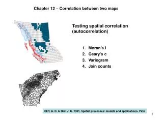
Joins Count Statistic Real World Uses? • Was the spatial pattern of 2000 Bush-Gore electoral outcomes random? • Build an adjacency matrix (49 x 49)
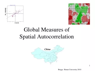
- - - Σ(yi-y)2 ΣΣwij(yi-y)(yj-y) n I = ΣΣwij Other Measures of Spatial Autocorrelation Moran’s I • Translates nonspatial correlation measures to spatial context • Applied to numerical ratio or interval data • Evaluates summed covariances corrected for sample size • I < 0, Negative Autocorrelation • I > 0, Positive Autocorrelation
- Σ(yi-y)2 ΣΣwij(yi-yj)2 n-1 C = 2ΣΣwij Other Measures of Spatial Autocorrelation Geary’s Contiguity Ratio C • Similar to Moran’s I • C = 1, No auto correlation • 0 < C < 1, Positive autocorrelation • C > 1 Negative autocorrelation
Other Measures of Spatial Autocorrelation Weighted Matrices • Weights can be added to calculations of Moran’s I or Geary’s C • e.g. weight state boundaries based on length of borders Lagged autocorrelation • weights in the matrix in which nonadjacent spatial autocorrelation is tested for. • e.g. CA and UT are neighbors at a lag of 2
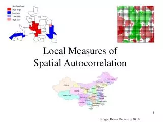
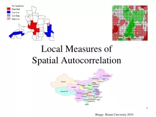
Local Indicators of Spatial Association (LISA) • Where are the data patterns within the study region? • Disaggregate measures of autocorrelation • Describe extent to which particular areal units are similar to their neighbors • Nonstationarity of data • When clusters of similar values found in specific sub-regions of study • Tests: G, I, &C