Download
1 / 20
220 likes | 458 Views
Autocorrelation and Heteroskedasticity. Introduction. Assess the main ways of remedying autocorrelation Describe the problem of non-constant error terms Assess the main test for heteroskedasticity Examine the main remedies for heteroskedasticity

E N D
Introduction • Assess the main ways of remedying autocorrelation • Describe the problem of non-constant error terms • Assess the main test for heteroskedasticity • Examine the main remedies for heteroskedasticity • Introduce the multivariate approach to regression analysis
Cochrane-Orcutt methodology • This approach to remedying autocorrelation relies on the generalised difference equation approach • It is an iterative procedure, the estimates of the parameters converge towards their actual value. • It assumes the autocorrelation follows a first order autoregressive process (simplest form)
Procedure (Based on previous slide) • Run regression and collect the error term (u). • Run a second regression of u against u(t-1) to obtain an estimate of ρ. • Form the generalised difference equation, to obtain new estimates of the parameters • Re-run this equation, obtain u and repeat process until there is no significant difference from one iteration to the next.
Restricted Version of the GDE • The generalised difference equation can be written in the following form, which includes a restriction, the product of the coefficients on y(-1) and x is equal to the negative of the coefficient on x(-1):
Unrestricted version of the GDE • In the unrestricted version of the equation in the previous slide, there are no restrictions on the values of the coefficients:
The Common Factor Test • To determine whether the restricted or unrestricted versions are best, we can use the common factor test, under the null hypothesis that the restriction holds, the test statistic is:
Heteroskedasticity • This occurs when a Gauss-Markov assumption is broken, it indicates non-constant variance of the error term. • It is often caused by variables which have substantial differences in the values of the observations, i.e. GDP differing between the USA and Cuba • With heteroskedasticity the estimator is no longer BLUE, as it is not the best.
Tests for Heteroskedasticity • Goldsfeldt-Quandt test (not used much now) • Whites Test (used in E-views computer software). • LM test (Similar to the LM test for heteroskedasticity)
White’s Test • This test follows a similar pattern to the LM test for autocorrelation discussed earlier. • Based on the same first equation as in slide 4, we estimate the model and collect the residual u. • Square the residual to form the variance of the residual • Run a secondary regression of the squared residual on the explanatory variable and this variable squared
White’s Test • This secondary regression appears like the following:
White’s Test • Collect the R-squared statistic and multiply by the number of observations to obtain the test statistic. • This follows a chi-squared distribution, the d of f equal the number of parameters in the secondary regression (i.e. 2 in above example) • The null hypothesis is no heteroskedasticity. • If there were 2 explanatory variables, you could include the cross product of these variables, in the secondary regression.
Remedies for heteroskedasticity • If the standard deviation of the residual is known, the heteroskedasticity can be removed by dividing the regression equation through by the standard deviation of the residual (weighted Least Squares) • If this is not known, as is likely, we need to stipulate what the standard deviation is equal to. We can then divide the regression equation through by this variable to obtain a constant variance residual.
Remedying Heteroskedasticity • If we assume the error variance is proportional to x, the explanatory variable and we have the usual model:
Remedying Heteroskedasticity • If we divide our model through by the square root of x:
Remedying Heteroskedasticity • Taking the new error term, we can show it is no longer suffering from heteroskedasticity by proving it is now constant:
Multivariate Regression • Regressions with more than one explanatory variable are similar to the bi-variate case, we can interpret the coefficients and t-statistics in much the same way as before. • We now have a potential problem with multicollinearity, when the explanatory variables are correlated • The formula for the β contains an expression for the covariance between the explanatory variables.
Multivariate Regression Analysis • The regression coefficients are more likely to be accurate, the less closely related are the explanatory variables • This allows testing for the significance of groups of variables • The R-squared increases with the more explanatory variables • We need to consider whether all relevant effects are included in the model • When estimating the t-tests, we need to account for the extra degrees of freedom • There is a trade off between the number of explanatory variables and the ease of interpreting the model
Conclusion • The common factor test can be used to determine the best solution to the problem of autocorrelation • In the presence of heteroskedasticity, the estimator is no longer BLUE. • White’s test is the most common test for heteroskedasticity • Weighted Least Squares can be used to remedy the heteroskedasticity problem.