Autocorrelation
Autocorrelation. Lecture 20. Today’s plan. Definition and implications How to test for first order autocorrelation Note: we’ll only be taking a detailed look at 1st order autocorrelation, but higher orders exist e.g. quarterly data is likely to have 4th order autocorrelation


Autocorrelation
E N D
Presentation Transcript
Autocorrelation Lecture 20
Today’s plan • Definition and implications • How to test for first order autocorrelation • Note: we’ll only be taking a detailed look at 1st order autocorrelation, but higher orders exist • e.g. quarterly data is likely to have 4th order autocorrelation • How to correct for first-order autocorrelation and how to estimate allowing for autocorrelation • Again we’ll use the Phillips curve as an example
Definitions and implications • Autocorrelation is a time-series phenomenon • 1st-order autocorrelation implies that neighboring observations are correlated • the observations aren’t independent draws from the sample
Definitions and implications (2) • In terms of the Gauss-Markov (or BLUE) theorem: • The model is still linear and unbiased if autocorrelation exists:
Definitions and implications (3) • Autocorrelation will affect the variance: • if s = t, then we would have: • but if s t, and Y observations are not independent, we have nonzero covariance terms:
Definitions and implications (4) • Think of a numerical example to demonstrate this • assuming t = 3: if we wanted to estimate : • We want to consider the efficiency, or the variance of • If BLUE: all covariance terms are zero. • If covariance terms are nonzero: we no longer have minimum variance • minimum variance is defined as
Summary of implications 1) Estimates are linear and unbiased 2) Estimates are not efficient. We no longer have minimum variance 3) Estimated variances are biased either positively or negatively 4) Unreliable t and F test results 5) Computed variances and standard errors for predictions are biased • Main idea: autocorrelation affects the efficiency of estimators
How does autocorrelation occur? Autocorrelation occurs through one of the following avenues: 1) Intertia in economic series through construction • With regards to unemployment this was called hysteresis: this means that certain sections of society who are prone to unemployment 2) Incorrect model specification • There might be missing variables or we might have transformed the model to create correlation across variables
How does autocorrelation occur? 3) Cobweb phenomenon • agents respond to information with lags to • this is usually related to agricultural markets 4) Data manipulation • example: constructing annual information based on quarterly data
Graphical results • With no autocorrelation in the error term: we would expect all errors to be randomly dispersed around zero within reasonable boundaries • Simply graphing the estimated errors against time indicates the possibility of autocorrelation: • we look for patterns of errors over time • patterns can be positive, negative, or zero • Graph error vs. time, we have positive correlation in the error term • errors from one time period to the next tend to move in 1 direction, with a positive slope
Phillips Curve • L_20.xls : Phillips Curve data • Can calculate predicted wage inflation using the observed unemployment rate and the estimated regression coefficients • Can then calculate the estimated error of the regression equation • Can also calculate the error lagged one time period
Durbin-Watson statistic • We will use the Durbin-Watson statistic to test for autocorrelation • This is computed by looking over T-1 observations where t = 1, …T
Durbin-Watson statistic (2) • The assumptions behind the Durbin-Watson statistic are: 1) You must include an intercept in the regression 2) Values of X are independent and fixed 3) Disturbances, or errors, are generated by: • this says that errors in this time period are correlated with errors in the last time period and some random error vt • is the coefficient of autocorrelation and is bounded -1 1 • can be calculated as
How to estimate • This estimation matters because it will be used in the model correction • can be estimated by this equation: • Once we have the Durbin-Watson statistic d, you can obtain an estimate for
How to estimate (2) • How the test works: • The values for d range between 0 and 4 with 2 as the midpoint • using :
indeterminate indeterminate 0 2 4 dL dU 4-dU 4-dL H0: =0 H1 H1 Reject null Reject null Cannot reject null How to estimate (3) • We can represent this in the following figure: • dL represents the D-W upper bound • dU represents the D-W lower bound • The mirror image of dL and dU are 4- dL and 4-dU
Procedure Table on the second handout for today is the Durbin-Watson statistical table and an additional table for this analysis 1) Run model: 2) Compute: 3) Compute d statistic 4) Find dL and dU from the tables K’ is the number of parameters minus the constant and T is the number of observations 5) Test to see if autocorrelation is present
0 2 4 0.331 1.475 dL 4-dU 4-dL dU H0: =0 H1 H1 Reject null Reject null Accept null Example (2) • Returning to L_20.xls
Generalized least squares • What can we do about autocorrelation? • Recall that our model is: Yt = a + bXt + et (1) • We also know: et = et-1 + vt • We will have to estimate the model using generalized least squares (GLS)
Generalized least squares (2) • Let’s take our model and lag it by one time period: Yt-1 = a + bXt-1 + et-1 • Multiplying by : Yt-1 = a + bXt-1 + et-1 (2) • Subtracting our (2) from (1), we get Yt - Yt-1 = a(1-) + b(Xt-1 - Xt-1) + vt where vt = et - et-1
Generalized least squares (3) • Now we need an estimate of : we can transform the variables such that: where: • Estimating equation (3) allows us to estimate without first-order autocorrelation
Estimating • There are several approaches • One way is by using a short cut: thinking back to the Durbin-Watson statistic, we can rewrite the expression for d as:
Estimating (2) • Collecting like terms, we have: • Solving for , we can get an estimate in terms of d: • Since earlier we defined as: • we can use this to get a more precise estimate • There are three or four other methods in the text