Download
1 / 24
250 likes | 393 Views
Magnetic Disk Characteristics I/O Connection Structure Types of Buses Cache & I/O I/O Performance Metrics I/O System Modeling Using Queuing Theory Designing an I/O System RAID (Redundant Array of Inexpensive Disks). (Chapter 7.5). RAID (Redundant Array of Inexpensive Disks).

E N D
Magnetic Disk Characteristics • I/O Connection Structure • Types of Buses • Cache & I/O • I/O Performance Metrics • I/O System Modeling Using Queuing Theory • Designing an I/O System • RAID (Redundant Array of Inexpensive Disks) (Chapter 7.5)
RAID (Redundant Array of Inexpensive Disks) • The term RAID was coined in a 1988 paper by Patterson, Gibson and Katz of the University of California at Berkeley. • In that article, the authors proposed that large arrays of small, inexpensive disks --usually SCSI, IDE support recently started-- could be used to replace the large, expensive disks used on mainframes and high-end servers. • In such arrays files are "striped" and/or mirrored across multiple drives. • Their analysis showed that the cost per megabyte could be substantially reduced, while both performance (throughput) and fault tolerance could be increased. • The Catch: Array Reliability without any redundancy : Reliability of N disks = Reliability of 1 Disk ÷ N 50,000 Hours ÷ 70 disks = 700 hours • Disk system MTTF: Drops from 6 years to 1 month! • Arrays (without redundancy) too unreliable to be useful! MTTF = Mean Time To Failure
Manufacturing Advantages of Disk Arrays Disk Product Families Conventional: 4 disk form factors 14” 3.5” 5.25” 10” High End Low End Disk Array: 1 disk form factor 3.5”
RAID Subsystem Organization array controller host single board disk controller host adapter manages interface to host, DMA single board disk controller control, buffering, parity logic single board disk controller physical device control single board disk controller Striping software off-loaded from host to array controller No application modifications No reduction of host performance often piggy-backed in small format devices
Basic RAID Organizations • Non-Redundant (RAID Level 0) • Mirrored (RAID Level 1) • Memory-Style ECC (RAID Level 2) • Bit-Interleaved Parity (RAID Level 3) • Block-Interleaved Parity (RAID Level 4) • Block-Interleaved Distributed-Parity (RAID Level 5) • P+Q Redundancy (RAID Level 6) • Striped Mirrors (RAID Level 10)
Non-Redundant Striped(RAID Level 0) • RAID 0 simply stripes data across all drives (minimum 2 drives) to increase data throughput but provides no fault protection. • Sequential blocks of data are written across multiple disks in stripes, as follows: • The size of a data block, which is known as the "stripe width” or unit, varies with the implementation, but is always at least as large as a disk's sector size. (typical stripe width 16-128 KBytes ) • This scheme offers the best write performance since it never needs to update redundant information. • It does not have the best read performance. • Redundancy schemes that duplicate data, such as mirroring, can perform better on reads by selectively scheduling requests on the disk with the shortest expected seek and rotational delays. Strictly speaking: Not really a RAID level (no redundancy)
Optimal Size of Data Striping Unit(Applies to RAID Levels 0, 5, 6, 10) • Lee and Katz [1991] use an analytic model of non-redundant disk arrays to derive an equation for the optimal size of data striping unit. • They show that the optimal size of data striping is equal to: • Where: • P is the average disk positioning time, • X is the average disk transfer rate, • L is the concurrency, Z is the request size, and • N is the array size in disks. • Their equation also predicts that the optimal size of data striping unit is dependent only the relative rates at which a disk positions and transfers data, PX, rather than P or X individually. • Lee and Katz show that the optimal striping unit depends on request size; Chen and Patterson show that this dependency can be ignored without significantly affecting performance. • Typical optimal values of striping unit = 16 - 128 KBytes
Mirrored (RAID Level 1) • Utilizes mirroring or shadowing of data using twice as many disks as a non-redundant disk array. • Whenever data is written to a disk the same data is also written to a redundant disk, so that there are always two copies of the information. • When data is read, it can be retrieved from the disk with the shorter queuing, seek and rotational delays • If a disk fails, the other copy is used to service requests. • Mirroring is frequently used in database applications where availability and transaction rate are more important than storage efficiency.
Memory-Style ECC (RAID Level 2) • RAID 2 performs data striping with a block size of one bit or byte, so that all disks in the array must be read to perform any read operation. • A RAID 2 system would normally have as many data disks as the word size of the computer, typically 32. • In addition, RAID 2 requires the use of extra disks to store an error-correcting code for redundancy. • With 32 data disks, a RAID 2 system would require 7 additional disks for a Hamming-code ECC. • Such an array of 39 disks was the subject of a U.S. patent granted to Unisys Corporation in 1988, but no commercial product was ever released. • For a number of reasons, including the fact that modern disk drives contain their own internal ECC, RAID 2 is not a practical disk array scheme.
Bit-Interleaved Parity (RAID Level 3) • One can improve upon memory-style ECC disk arrays ( RAID 2) by noting that, unlike memory component failures, disk controllers can easily identify which disk has failed. Thus, one can use a single parity disk rather than a set of parity disks to recover lost information. • As with RAID 2, RAID 3 must read all data disks for every read operation. • This requires synchronized disk spindles for optimal performance, and works best on a single-tasking system with large sequential data requirements. An example might be a system used to perform video editing, where huge video files must be read sequentially.
Block-Interleaved Parity (RAID Level 4) • RAID 4 is similar to RAID 3 except that blocks of data are striped across the disks rather than bits/bytes. • Read requests smaller than the striping unit access only a single data disk. • Write requests must update the requested data blocks and must also compute and update the parity block. • For large writes that touch blocks on all disks, parity is easily computed by exclusive-or’ing the new data for each disk. • For small write requests that update only one data disk, parity is computed by noting how the new data differs from the old data and apply-ing those differences to the parity block. • This can be an important performance improvement for small or random file access (like a typical database application) if the application record size can be matched to the RAID 4 block size. Correction: Blocks not bits
Block-Interleaved Distributed-Parity (RAID Level 5) • The block-interleaved distributed-parity disk array eliminates the parity disk bottleneck present in RAID 4 by distributing the parity uniformly over all of the disks. • An additional, frequently overlooked advantage to distributing the parity is that it also distributes data over all of the disks rather than over all but one. • RAID 5 has the best small read, large read and large write performance of any redundant disk array. • Small write requests are somewhat inefficient compared with redundancy schemes such as mirroring however, due to the need to perform read-modify-write operations to update parity.
RAID-5: Small Write Algorithm 1 Logical Write = 2 Physical Reads + 2 Physical Writes D0 D1 D2 D0' D3 P old data new data old parity (1. Read) (2. Read) XOR + + XOR (3. Write) (4. Write) D0' D1 D2 D3 P' Problems of Disk Arrays: Small Writes
P+Q Redundancy (RAID Level 6) • An enhanced RAID 5 with stronger error-correcting codes used . • One such scheme, called P+Q redundancy, uses Reed-Solomon codes, in addition to parity, to protect against up to two disk failures using the bare minimum of two redundant disks. • The P+Q redundant disk arrays are structurally very similar to the block-interleaved distributed-parity disk arrays (RAID 5) and operate in much the same manner. • In particular, P+Q redundant disk arrays also perform small write operations using a read-modify-write procedure, except that instead of four disk accesses per write requests, P+Q redundant disk arrays require six disk accesses due to the need to update both the ‘P’ and ‘Q’ information.
Increasing Logical Disk Addresses D0 D1 D2 D3 P A logical write becomes four physical I/Os Independent writes possible because of interleaved parity Reed-Solomon Codes ("Q") for protection during reconstruction D4 D5 D6 P D7 D8 D9 P D10 D11 D12 P D13 D14 D15 Stripe P D16 D17 D18 D19 Targeted for mixed applications Stripe Unit D20 D21 D22 D23 P . . . . . . . . . . . . . . . Disk Columns RAID 5/6: High I/O Rate Parity
RAID 10 (Striped Mirrors) • RAID 10 (also known as RAID 1+0) was not mentioned in the original 1988 article that defined RAID 1 through RAID 5. • The term is now used to mean the combination of RAID 0 (striping) and RAID 1 (mirroring). • Disks are mirrored in pairs for redundancy and improved performance, then data is striped across multiple disks for maximum performance. • In the diagram below, Disks 0 & 2 and Disks 1 & 3 are mirrored pairs. • Obviously, RAID 10 uses more disk space to provide redundant data than RAID 5. However, it also provides a performance advantage by reading from all disks in parallel while eliminating the write penalty of RAID 5.
RAID Levels Summary Minimum number of RAID Level disk faults Example Corresponding Widely survived Data Disks Check Disks Used? 0 Non-Redundant Striped 0 8 0 Yes 1 Mirrored 1 8 8 No 10 Striped Mirrors 1 8 8 Yes 2 Memory-Style ECC 1 8 4 No 3 Bit-Interleaved Parity 1 8 1 No 4 Block-Interleaved Parity 1 8 1 No 5 Block-interleaved 1 8 1 yes Distributed Parity 6 P + Q Redundancy 2 8 2 No
RAID Levels Comparison:Throughput Per Dollar Relative to RAID Level 0.
RAID Levels Comparison:Throughput Per Dollar Relative to RAID Level 0.
RAID Levels Comparison:Throughput Per Dollar Relative to RAID Level 0.
RAID Levels Comparison:Throughput Per Dollar Relative to RAID Level 0.
RAID Reliability • Redundancy in disk arrays is motivated by the need to overcome disk failures. • When only independent disk failures are considered, a simple parity scheme works admirably. Patterson, Gibson, and Katz derive the mean time between failures for a RAID level 5 to be: MTTF (disk)2 / N (G - 1) MTTR(disk) • where MTTF(disk) is the mean-time-to-failure of a single disk, • MTTR(disk) is the mean-time-to-repair/replace of a single disk, • N is the total number of disks in the disk array • G is the parity group size • For illustration purposes, let us assume we have: • 100 disks that each had a mean time to failure (MTTF) of 200,000 hours and a mean time to repair of one hour. If we organized these 100 disks into parity groups of average size 16, then the mean time to failure of the system would be an astounding 3000 years! • Mean times to failure of this magnitude lower the chances of failure over any given period of time.
Array Controller String Controller . . . String Controller . . . String Controller . . . String Controller . . . String Controller . . . String Controller . . . Data Recovery Group: unit of data redundancy System Availability: Orthogonal RAIDs Redundant Support Components: power supplies, controller, cables
System-Level Availability host host Fully dual redundant I/O Controller I/O Controller Array Controller Array Controller . . . . . . . . . Goal: No Single Points of Failure . . . . . . . . . with duplicated paths, higher performance can be obtained when there are no failures Recovery Group