Download
1 / 22
220 likes | 357 Views
Ocean Overview Science, Applications, & Observation Requirements. Chuck McClain GeoCAPE Workshop August 18-20, 2008. Nanticoke. Patuxent. Wicomico. Potomac. Pocomoke. Rappahannock. York. SeaWiFS 1.1 km. James. Chl-a (mg/m 3 ). MODIS 250 m False Color. Chesapeake Bay. Oregon.

E N D
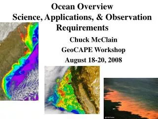
Ocean OverviewScience, Applications, & Observation Requirements Chuck McClain GeoCAPE Workshop August 18-20, 2008
Nanticoke Patuxent Wicomico Potomac Pocomoke Rappahannock York SeaWiFS 1.1 km James Chl-a (mg/m3) MODIS 250 m False Color Chesapeake Bay
Oregon California “Mesoscale” Biological Variability: U.S. West Coast
SeaWiFS, MODIS, & VIIRS • SeaWiFS • Rotating telescope • 412, 443, 490, 510, 555, 670, 765, 865 nm bands • 12 bit digitization truncated to 10 bits on spacecraft • 4 focal planes, 4 detectors/band, 4 gain settings, bilinear gain configuration • Polarization scrambler: sensitivity at 0.25% level • Solar diffuser (daily observations) • Monthly lunar views at 7° phase angle via pitch maneuvers • NPP/VIIRS (Ocean Color) • SeaWiFS-like rotating telescope • MODIS-like focal plane arrays (16 detectors/band) • 12 bit digitization • No polarization scrambler • Solar diffuser with stability monitor • 7 OC bands (412, 445, 488, 555, 672, 746, 865 nm) • Dual gains except 746 nm (single gain) • Monthly lunar views at 55° phase angle via space view port with roll maneuvers (feasible, but not approved) • MODIS (Ocean Color) • Rotating mirror • 413, 443, 488, 531, 551, 667, 678, 748, 870 nm bands • Single gain (NIR saturation) • 12 bit digitization • 4 focal planes (7-11 bands each) • OC Visible: 412-547 nm (5 bands-10 detectors each) • OC NIR: 667-869 (4 bands-10 detectors each) • No polarization scrambler: sensitivity at ~3% level • Spectral Radiometric Calibration Assembly (SRCA) • Solar diffuser (observations every orbit), Solar Diffuser Stability Monitor (SDSM) • Monthly lunar views at 55° phase angle via space view port Sensor designs & performance are never identical.
300 400 500 600 700 800 900 MODIS Bands 748 547 869 532 667 443 412 490 678 2135 1640 1240 NIR/SWIR: Atmospheric correction/ Coastal/Turbid Water VISIBLE: Taxonomy Pigment biomass Diffuse Attenuation + Solar calibration (spectral & temporal) + Lunar calibration (temporal) + Comprehensive Cal/Val (inc. vicarious cal sites) ULTRAVIOLET: Colored Dissolved Organic Matter Particulate scattering Atmospheric correction
Chlorophyll-a CH3 Quantifying Phytoplankton Processes from Space From chlorophyll absorption to chlorophyll concentration via optics Chlorophyll Algorithm SeaWiFS Marine Spectral Reflectance
Historical Ocean Color Accuracy Goals:Open Ocean • Sensor radiometric calibration • ±5% absolute • ±1% band-to-band relative • Water-leaving radiances • ±5% absolute • Chlorophyll-a • ±35% over range of 0.05-50.0 mg/m3 Revised requirements should be ~ 0.5% and 0.1% respectively. Current Ocean Biogeochemistry CDRs. These accuracy specifications need to be redefined to reflect future ocean science product accuracy requirements
Ocean Biology/Biogeochemistry Science Overview (cont’d) 2007 Advanced Plan for NASA’s Ocean Biology and Biogeochemistry Program Four key science questions requiring new observations: • “How are oceanecosystemsand thebiodiversitythey support influenced by climate and environmental variability and change, and how will these changes occur over time?” Ocean phytoplankton have a profound influence on the global carbon cycle. Important groups, such these calcifying phytoplankton in the Bering Sea, are seriously threatened by climate change. • “How docarbonand otherelementstransition between ocean pools and pass through the Earth System, and how do biogeochemical fluxes impact the ocean and Earth's climate over time?” • “How (and why) is the diversity and geographical distribution of coastal marinehabitats changing, and what are the implications for the well-being of human society?” Harmful algae that cause ‘red tides’ are a serious health hazard for humans. They are now more frequent and widely dispersed. • “How dohazards and pollutants impact the hydrography and biology of the coastal zone? How do they affect us, and can we mitigate their effects?”
Sustainability Feedbacks Ocean Biology/Biogeochemistry Research Goals to Observations ACE Ocean Radiometer ACE Ocean Radiometer Observations trace directly to Science Goals * UV * Short UV for advanced atmospheric correction Ocean Biology & Biogeochemistry Plan Key Biochemistry & Biology Properties NASA Strategic Plan Visible • Dissolved carbon • Phytoplankton pigments • Functional groups • Physiology • Particle size • Calcite • Fluorescence • Coastal biology • Atmospheric corrections* 98 bands from 335 – 865 nm, 19 aggregate bands total • Ecosystems & biodiversity • Carbon/elemental cycles • Habitats • Hazards • Understand Earth system • New observations to detect and predict change NIR Key environmental parameters Research objectives for Earth Science Ocean biology and biogeochemistry questions Measurement requirements lead to lead to lead to SWIR
Ocean Products • Current Global Products • Normalized water-leaving radiances (visible bands) • Chlorophyll-a concentration • Colored dissolved organic matter • Primary productivity • Diffuse attenuation @ 490 nm • Photosynthetically available radiation • Calcite concentration • Fluorescence line height (MODIS only) • Particulate organic carbon (next reprocessing) • Inherent optical properties (absorption and scattering coefficients) • Regionally-specific Products • Dissolved organic carbon concentration • Harmful algal bloom detection/spatial extent • …and others • Additional Future Products (Decadal Survey ocean sensors) • Phytoplankton functional groups • Particle size distributions • Habitat classifications • …others SeaWiFS & MODIS spectral bands limit the accuracy and variety of marine data products, particularly in coastal regions.
Calibration/Validation Paradigm Program Elements: • Laboratory - prelaunch sensor calibration & characterization • On-orbit - solar and lunar observations are used to track changes in sensor response • Field - comparison of satellite data retrievals to in-water, above-water and atmospheric observations • Vicarious calibration - adjust instrument gains to match water-leaving radiances • Product validation (water-leaving radiances, chl-a, etc.)
SeaWiFS Temporal Degradation Once a month, the SeaWiFS satellite (Orbview-2) is pitched to observe the Moon at a phase angle ~ 7° to track sensor sensitivity loss.
Vicarious Calibration Marine Optical Buoy (MOBY) is used to adjust prelaunch calibration for visible bands using satellite-buoy comparisons. Only a small % of samples result in a MOBY-satellite “match-up” for the “vicarious calibration”. MOBY Water-leaving Radiance Time Series (1997-2000)
Issues in Coastal Regions • Variety of aerosol types & atmospheric corrections • High reflectance in NIR (induces errors in aerosol radiance estimation) • NO2 absorption at UV and blue wavelengths • High SNR requirements (low ocean radiances in UV, visible, & NIR) • Dissolved organic materials & suspended sediments • Bottom influences on water-leaving radiances • Adjacency effects (scattered light from nearby bright land features) • Collection of high quality field data in turbid water • Quantification of spatial and temporal variability of marine properties and processes
Synergisms: Ocean & Atmospheric Sciences in Coastal Regions • Aerosol loading and properties • Ocean atmospheric corrections • Ozone & NO2 concentrations • Ocean atmospheric corrections • Surface reflectances • Ocean & atmosphere derived products • Air-sea gas exchanges • CO2 • Atmospheric nitrogen sources (nutrients) • UV bands • Ocean pigment discrimination • Atmospheric corrections • Cross-calibration with LEO sensors
mW cm2 sr m U.S. East Coast April 28, 2003 Green wavelength 551 nm Total top-of-the-atmosphere radiance 0 – 4
mW cm2 sr m Green wavelength 551 nm Total top-of-the-atmosphere radiance corrected for ozone absorption and Rayleigh (gas molecule) scattering 0 – 4
mW cm2 sr m Green wavelength 551 nm Total top-of-the-atmosphere radiance corrected for ozone absorption, Rayleigh & aerosol scattering 0 – 4
mW cm2 sr m Green wavelength 551 nm Normalized water-leaving radiance 0 – 2
Chlorophyll-a concentration 0 – 64 mg / m3
upper middle lower Chesapeake Bay Chesapeake Bay Chlorophyll-a Retrievals MODIS SWIR-based vs. NIR-based aerosol corrections Chlorophyll (mode) Field: 10 mg/m3 w/o SWIR: 22 mg/m3 w/ SWIR: 8 mg/m3 Field: 8 mg/m3 w/o SWIR: 16 mg/m3 w/ SWIR: 6 mg/m3 Field: 6 mg/m3 w/o SWIR: 8 mg/m3 w/ SWIR: 6 mg/m3