2D Movement Pathfinding
370 likes | 535 Views
This lecture explores 2D movement and pathfinding techniques essential for game development. It begins with methods for path following using Lerp and Catmull-Rom interpolation, addressing the challenge of perceived speed based on distance. A solution is proposed for consistent movement speed based on unit speed and distance. It discusses pathfinding algorithms, including the All Pairs Shortest Path (APSP) and A* algorithm, emphasizing their importance in navigating dynamic game environments. Learn how to implement these techniques to enhance player and AI interactions in games.

2D Movement Pathfinding
E N D
Presentation Transcript
2D Movement Pathfinding
Path Following at Constant Speed • In previous lecture showed path following • Used Lerp and CatmullRom interpolation methods built into Vector2 class • These methods take an amount • A number between 0 and 1 indicating the percentage distance between the start and end points (a “weight”) • Problem • A given amount can result in different perceived speeds, depending on the length of the line • Solution • Given a desired speed in terms of units per clock tick • Compute per-tick change in amount as follows • Per-tick-amount = unit-speed / Vector2.Distance(start, end) • That is, determine the percentage of the total distance between the points covered by one unit-speed
Pathfinding • In many games, computer controlled opponents need to move from one place to another in the game world • If the start and end points are known in advance, and never change, • Can simply define a fixed path • Computed before the game begins • Use path following techniques from previous lecture • Most platformers do this • If the start and end points vary, and are not known in advance (or may vary due to changes in game state), • Have to compute the path to follow while the game is running • Need to use a pathfinding algorithm Video of pathfinding problems Pathfinding Article: http://www.ai-blog.net/archives/000152.html
Pathfinding Representations • Waypoints • Navigation Meshes
All Pairs Shortest Path (APSP) • Assume a labeled directed graph • Nodes are pathnodes in your map • Labels are the distances between connecting nodes (or other specific cost information) • G=(V, E) in which each arc v → w has a non-negative cost C[v,w]. • Find, for each ordered pair (v,w) the smallest length of any path from v to w.
All Pairs Shortest Path (APSP) Floyd’s Algorithm • Assume the vertices in V are numbered 1,...,n. • Use an n X n matrix in which to compute the lengths of the shortest paths.
All Pairs Shortest Path (APSP) Floyd’s Algorithm • Set A[i,j] = C[i,j] for all i not equal to j. • If there is no arc from i to j, then assume C[i,j] = ∞. • Each diagonal element is set to 0.
All Pairs Shortest Path (APSP) Floyd’s Algorithm • Make n iterations over the matrix • On the kth iteration, A[i,j] will have for its value the smallest length of any path from i to j that doesn’t pass through a vertex numbered higher than k.
All Pairs Shortest Path (APSP) Floyd’s Algorithm • On the kth iteration, use the following formula to compute A Ak-1[i,j] • A[i,j] = min{ Ak-1[i,k] + Ak-1[k,j]
All Pairs Shortest Path (APSP) Floyd’s Algorithm • On the kth iteration, use the following formula to compute A Ak-1[i,j] • A[i,j] = min{ Ak-1[i,k] + Ak-1[k,j] The cost of going from i to j without going through k or any higher node
All Pairs Shortest Path (APSP) Floyd’s Algorithm • On the kth iteration, use the following formula to compute A Ak-1[i,j] • A[i,j] = min{ Ak-1[i,k] + Ak-1[k,j] The cost of going from i to k, then k to j, without going through any node higher than k.
Floyd Example 8 A0[i,j] 2 2 1 2 3 3 5
Floyd Example 8 A1[i,j] 2 2 1 2 3 3 5
Floyd Example 8 A1[i,j] 2 2 1 2 3 3 5
Floyd Example 8 A1[i,j] 2 2 1 2 3 3 5
Floyd Example 8 A1[i,j] 2 2 1 2 3 3 5
Floyd Example 8 A2[i,j] 2 2 1 2 3 3 5
Floyd Example 8 A2[i,j] 2 2 1 2 3 3 5
Floyd Example 8 A2[i,j] 2 2 1 2 3 3 5
Floyd Example 8 A2[i,j] 2 2 1 2 3 3 5
Floyd Example 8 A3[i,j] 2 2 1 2 3 3 5
Floyd Example 8 A3[i,j] 2 2 1 2 3 3 5
Floyd Example 8 A3[i,j] 2 2 1 2 3 3 5
Floyd’s Code Aho, Hopcroft and Ullman, Data Structures and Algorithms, Addison Wesley, pages 208-213. Including code for keeping track of the actual paths! CSC481 Design and Development of Computer Games
A* pathfinding • A* algorithm is widely used as the conceptual core for pathfinding in computer games • Most commercial games use variants of the algorithm tailored to the specific game • Original paper: • A Formal Basis for the Heuristic Determination of Minimum Cost Paths • Hart, P.E.; Nilsson, N.J.; Raphael, B. • IEEE Trans. Systems Science and Cybernetics, 4(2), July 1968, pp. 100-107 • A* is a graph search algorithm • There is a large research literature on graph search algorithms, and computer game pathfinding
Overview of A* algorithm • The following slides borrow heavily from: • A* Pathfinding for Beginners, by Patrick Lester • http://www.policyalmanac.org/games/aStarTutorial.htm • Problem • A unit wants to move from point A to point B on a game map, ideally along the shortest path • Assume the game map is a rectangular grid • Makes explanation easier, algorithm can accommodate many grid types • The literature views the map as a graph • Map squares are • Open/walkable (open terrain) • Or closed/unwalkable (walls, water, etc.)
Running Example • A unit in the green square wants to move to the red square • From here on out, we’ll call the squares “nodes” to be consistent with the research literature • Moving • Horizontally or vertically requires 10 movement points • Diagonal movement requires 14 movement points • Cannot move through blue squares (wall, unwalkable) • Observations • Can’t just draw a line between A and B and follow that line • Wall in-between • It’s not ideal to just follow the minimal line between A and B until you hit the wall, then walk along wall • Not an optimal path Pathfinding example.Green square is starting location, red square is desired goal. Blue is a wall. Black is walkable, blue is unwalkable.
Open and Closed Lists • Starting the search • Add A to open list of nodes to be considered • Look at adjacent nodes, and add all walkable nodes to the open list • I.e., ignore walls, water, or other illegal terrain • For each of these squares, note that their parent node is the starting node, A • Remove A from open list, add to closed list • Open list • Contains nodes that might fall along the path (or might not) • A list of nodes that need to be “checked out” • Closed list • A list of nodes that no longer need to be considered State of A* after the first step has completed. All adjacent nodes are part of the open list. The circle with line points to the parent node. The blue outline around the green start node indicates it is in the closed list.
Where to go next… • Now need to determine which node to consider next • Do not want to consider all nodes, since the number of nodes expands exponentially with each square moved (bad) • Want to pick the node that is closest to the destination, and explore that one first • Intuitive notion of “closest” • Add together: • The cost we have paid so far to move to a node (“G”) • An estimate of the distance to the end point (“H”)
Computing the cost • F=G+H • Movement cost to get to destination • G • Movement cost to move from start node A to a given node on the grid • Following the path generated to get there • Add 10 for horizontal/vertical move, 14 for diagonal move • H • Estimated movement cost to move from that given node on the grid to the final destination, node B • Known as the heuristic • A guess as to the remaining distance • There are many ways to make this guess—this lecture shows just one way
Computing H using Manhattan method • Manhattan method • Calculate the total number of nodes moved horizontally/vertically to reach the target node (B) from the current square • Ignore diagonal movement, and ignore obstacles that may be in the way. • Multiply total # of nodes by 10, the cost for moving one node horizontally/vertically. • Called Manhattan method because it is like calculating the number of city blocks from one place to another, where you can’t cut across the block diagonally. After first step, showing costs for each node.G = movement cost to reach the current node (lower left)H = Manhattan estimate of cost to reach the destination from node (lower right)F = G + H (total cost)
Continuing the search • Pick the node with lowest F value • Drop it from open list, add to closed list • Check adjacent nodes • Add those that are walkable, and not already on open list • The parent of the added nodes is the current node • If an adjacent nodes is already on the open list, check to see if this path to that node is a better one. • Check if G score for that node is lower if we use the current node to get there. If not, don’t do anything. • On the other hand, if G cost of new path is lower change the parent of the adjacent square to the selected square • (in the diagram, change the direction of the pointer to point at the selected square) • Finally, recalculate both the F and G scores of that square. After picking node with lowest F value. Node is in blue, indicating it is now in closed list.
Example Consider node to right. Check adjacent squares. Ignore starting point (on closed list). Ignore walls (unwalkable). Remaining nodes already on open list, so check to see if it is better to reach those nodes via the current node (compare G values). G score is always higher going through current node. Need to pick another node. Go through list of open nodes, and pick one with lowest F cost. There are two choices with equal F cost. Pick the lower one (could have picked upper one). Check adjacent nodes. Ignore walls and closed list. Ignore diagonal under wall (game-specific corner rule). Add two new squares to open list (below and below diagonal). Check G value of path via remaining square (to left) – not a more efficient path.
Example continued Repeat process until target node is added to the closed list. Results in situation above. To determine final path, start at final node, and move backwards from one square to the next, following parent/child relationships (follow arrows).
Some issues • Collision avoidance • Need to avoid other units in the game • One approach: make squares of non-moving units unwalkable • Can penalize nodes on movement paths of other units • Variable terrain cost • In many games, some terrain costs more to move over than others (mountains, hills, swamps) • Change movement costs for these terrains • But, can cause units to preferentially choose low-cost movement paths • Example: units always go through mountain pass, and then get whacked by big unit camping at exit • Add influence cost to nodes where many units have died
More issues • Unexplored areas • Pathfinding can make units “too smart” since their movement implies knowledge of unmapped areas of the map • Have a knownWalkable array for explored areas • Mark rest of the map as walkable, until proven otherwise • Memory/speed • Algorithm can use a lot of memory • Can also slow things down • Spread A* computations over many game ticks
