Download
1 / 48
480 likes | 646 Views
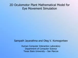
2D Oculomotor Plant Mathematical Model for Eye Movement Simulation. Sampath Jayarathna and Oleg V. Komogortsev Human Computer Interaction Laboratory Department of Computer Science Texas State University – San Marcos . Motivation.

E N D
2D Oculomotor Plant Mathematical Model for Eye Movement Simulation • Sampath Jayarathna and Oleg V. Komogortsev Human Computer Interaction Laboratory Department of Computer Science Texas State University – San Marcos
Motivation • Accurate eye movement prediction will increase the responsiveness of every system that uses eye-gaze-based commands. • As an example, prediction of fast eye movement (saccade) will allow placing system’s response to the area targeted by a saccade, anticipating a user’s intentions.
Objectives The main objective of this research is to extend the work proposed by horizontal 2DOPMM by designing a framework that predicts an eye movement trajectory in any direction within a specified time interval, detects saccades, provides an eye position signal during periods when the eye tracking fails, and has a real-time performance.
Proposed Contribution An eye mechanical model that is capable of generating saccades that start from any direction of eye position and progress in any direction in Listing’s plane. The representation of the eye mechanical model in a Kalman Filter form. This representation enables continuous real-time eye movement prediction.
Previous Work • Our model grows from the horizontal OPMM by addition of two extraocular muscles (superior/inferior rectus) and allowing vertical eye movements. • The horizontal OPMM accounts for individual anatomical components (passive elasticity, viscosity, eye-globe rotational inertia, muscle active state tension, length tension characteristics, force velocity relationship) and considers each extraocular muscle separately, therefore allowing estimation of individual extraocular muscle force values.
Previous Work… • When compared to three-dimensional models, our model accounts for individual anatomical properties of extraocular muscles (lateral, medial, superior, and inferior rectus) and its surroundings stated earlier.
Human Visual System The eye globe rotates in its socket through the use of six muscles, lateral/medial recti- mainly responsible for horizontal eye movements, superior/inferior recti- mainly responsible for vertical eye movements, superior/inferior oblique – mainly responsible for eye rotation around its primary axis of sight, and vertical eye movements
Human Visual System…. • The brain sends a neuronal control signal to each muscle to direct the muscle to perform its work. • A neuronal control signal is anatomically implemented as a neuronal discharge that is sent through a nerve to a designated muscle from the brain. • During an eye movement, movement trajectory can be separated into horizontal and vertical components. • The neuronal control signal for the horizontal and vertical components is generated by different parts of the brain.
2D Oculomotor Plant Model • Our 2D OPMM is driven by the neuronal control signal innervating four extraocular muscles lateral, medial, superior, and inferior recti that induce eye globe movement. • The 2DOPMM resistive forces are provided by surrounding tissues.
2D Oculomotor Plant Model……. • Each muscle plays the role of the agonist or the antagonist. • The agonist muscle contracts and pulls the eye globe in the required direction and the antagonist muscle stretches and resists the pull [2]. • This research discusses in detail only Right Upward and Left Downward movements as examples, but the model can be modified to simulate eye globe movements in all directions.
2D Oculomotor Plant Model……. • Evoked by muscle movements, an eye can move in 8 different directions: • Right Horizontal • Left Horizontal • Top Vertical • Bottom Vertical • Right Upward • Left Upward • Right Downward • Left Downward
Right Upward Eye movement When eye moves to a particular position from the coordination position (0,0) as one of eight basic movement types listed above, each muscle connected to the eye globe contract or stretch accordingly. Lateral Rectus - ? Medial Rectus - ? Superior Rectus - ? Inferior Rectus - ?
Right Upward Eye movement….. Rotations of each muscle because of the horizontal and vertical displacement of the eye from its origin ΘHR and ΘVR , makes a rotation angle with respective to each of muscle connected to the eye globe, by lateral rectus, superior rectus, medial rectus and inferior rectus ΘLR, ΘSR, ΘMR, ΘIR respectively.
Right Upward eye movement….. When human eye rotates to a new target axis due to visual stimuli, each eye muscle is innervated by a neuronal control signal producing necessary muscle forces for each eye globe rotation with required direction and magnitude. By computing muscle forces as Horizontal Right, Horizontal Left, Vertical Top and Vertical Bottom, these forces can be defined based on muscle properties, and also later will allow to compute individual extraocular muscle forces.
Vertically & Horizontally projected muscle forces at Right Upward eye movement
Right Upward eye movement….. When mapped to the horizontal and vertical planes, each extraocular muscle provides a projection of its force. Those projections are directed according to original 2D movements, therefore creating 4 equations of forces in horizontal and vertical planes: Horizontal Right Muscle Force (THR_R_MF) : TLRCosΘLR Horizontal Left Muscle Force (THR_L_MF) : TMRCosΘMR+ TSRSinΘSR+ TIRSinΘIR Vertical Top Muscle Force (TVR_T_MF) : TSRCosΘSR Vertical Bottom Muscle Force (TVR_B_MF) : TIRCosΘIR+ TMRSinΘMR+ TLRSinΘLR
Individual Muscle Properties • Detailed computation of muscle forces requires accurate modeling of each component inside of an extraocular muscle. • These components are passive elasticity, an active state tension, series elasticity, a length tension component and a force velocity relationship. • Combined these components creates a Muscle Mechanical Model (MMM).
Individual Muscle Properties….. Passive Elasticity: Each body muscle in the rest state is elastic. The rested muscle can be stretched by applying force, the extension being proportional to the force applied. The passive muscle component is non-linear, but in this paper it is modeled as an ideal linear spring. Active State Tension: If stimulated by a single wave of neurons, a muscle twitches then relaxes. A muscle goes into the tetanic state, when its stimulated by a neurons at a specific frequency continuously [13]. When a tetanic stimulation occurs, a muscle develops tension, trying to contract. The resulting tension is called the active state tension.
Individual Muscle Properties….. Length Tension Relationship: The tension that a muscle develops as a result of neuronal stimulation partially depends on its length. In this paper the length tension relationship is modeled as an ideal linear spring. Series Elasticity: The series elasticity is in series with the active force generator, hence the name. In this 2DOPMM, the series elasticity is modeled as an ideal liner spring. Force Velocity Relationship: This dependency of force upon velocity varies for different levels of neuronal control signal and depends on whether a muscle shortens or being stretched.
Horizontal Right Muscle Force MMM at Fixation Neuronal control signal NLRcreates active tension force FHR_LR that works in parallel with the length-tension force FHR_LT_LR . Altogether they produce tension that is propagated through the series elasticity components to the eye globe.
MMM Scalar Values Length tension force of lateral rectus is, whereθHR_LT_LR is the displacement of the spring in the horizontal direction and KLT is the spring’s coefficient The force propagated by the series elasticity component is, whereθHR_SE_LR is the displacement of the spring in the horizontal direction and KSE is the spring’s coefficient.
Horizontal Right muscle force….. In this particular situation, lateral rectus behaves as agonist and hence shows agonist muscle properties with Horizontal Muscle force values. THR_R_MF = lateral rectus Active State Tension + lateral rectus Length Tension Component – lateral rectus Damping component Resisting the contraction, the series elasticity component of the lateral rectus propagates the contractile force by pulling the eye globe with the same force THR_R_MF , THR_R_MF = lateral rectus Series Elasticity Component
Horizontal Right muscle force….. The damping component modeling the force velocity relationship resists the muscle contraction. The amount of resistive force produced by the damping component is based upon the velocity of contraction of the length tension component.
Horizontal Right muscle force….. By using previous 2 equations, we can calculate the force THR_R_MF in terms of the eye rotation ∆ΘHR and displacement of the length tension component ∆ΘHR_LT_LR of the muscle.
Horizontal Left muscle force Medial Rectus - Antagonist Superior Rectus - Agonist Inferior Rectus - Antagonist
Horizontal Left muscle force….. THR_L_MF = TMR +TSR +TIR Values for the Force component of the superior rectus can be calculated as same way in the previous agonist muscle lateral rectus. Force components for the medial and inferior recti shows similar composition as antagonist muscles. TMR = - (medial rectus Active State Tension + medial rectus Length Tension Component + medial rectus Damping component) TMR = - medial rectus Series Elasticity Component
Horizontal Left muscle force….. Consider Medial Rectus Antagonist Muscle, Total Displacement θHR_MR θHR_MR increases when the eye moves to the right by ∆θHR, making the resulting displacement θHR_MR + ∆θHR Both length tension and series elasticity components lengthen as a result of the agonist pull.
Horizontal Left muscle force….. By similar method, we can obtain 2 major equations for the horizontal left muscle force using 6 muscle equations (2 equations for each muscle, medial, superior and inferior rectus). By using above 2 equations, we can calculate the force THR_L_MF in terms of the eye rotation ∆ΘHR , ∆ΘVRand displacement of the length tension components of the 3 muscles, ∆ΘHR_LT_MR , ∆ΘVR_LT_SR , and ∆ΘVR_LT_IR.
Vertical Top muscle forces By similar calculations, we can obtain Vertical Top Muscle Force where superior rectus behaves as agonist, with 2 more equations of forces, in terms of the eye rotation ∆ΘVR and displacement of the length tension component ∆ΘVR_LT_SR of the muscle.
Vertical Bottom muscle forces And also, in Vertical Bottom Muscle force, medial rectus and inferior rectus behave as antagonist, and lateral rectus behaves as agonist, by providing 2 muscle force values for the Vertical Bottom muscle force, in terms of the eye rotation ∆ΘHR , ∆ΘVR and displacement of the length tension components of the 3 muscles, ∆ΘHR_LT_MR , ∆ΘHR_LT_LR , and ∆ΘVR_LT_IR.
Active State Tension Active state tension appears as a result of the neuronal control signal send by the brain. In our 2DOPMM model, the active state tension is a result of a low pass filtering process performed upon the neuronal control signal. Active state tension dynamics can be represented with the following differential equations at each time interval both in horizontal and vertical planes
Active State Tension….. For Agonist, [𝑡𝑠𝑎𝑐 _𝑠𝑡𝑎𝑟𝑡 , 𝑡𝐴𝐺_𝑠𝑎𝑐 _𝑝𝑢𝑙𝑠𝑒 _𝑠𝑡𝑎𝑟𝑡 ], [𝑡𝐴𝐺_𝑠𝑎𝑐 _𝑝𝑢𝑙𝑠𝑒 _𝑠𝑡𝑎𝑟𝑡 , 𝑡𝐴𝐺_𝑠𝑎𝑐 _𝑝𝑢𝑙𝑠𝑒 _𝑒𝑛𝑑 ], [𝑡𝐴𝐺_𝑠𝑎𝑐 _𝑝𝑢𝑙𝑠𝑒 _𝑒𝑛𝑑 , 𝑡𝑠𝑎𝑐 _𝑒𝑛𝑑 ] For Antagonist [𝑡𝑠𝑎𝑐 _𝑠𝑡𝑎𝑟𝑡 , 𝑡𝐴𝑁𝑇_𝑠𝑎𝑐 _𝑝𝑢𝑙𝑠𝑒 _𝑠𝑡𝑎𝑟𝑡 ], [𝑡𝐴𝑁𝑇_𝑠𝑎𝑐 _𝑝𝑢𝑙𝑠𝑒 _𝑠𝑡𝑎𝑟𝑡 , 𝑡𝐴𝑁𝑇_𝑠𝑎𝑐 _𝑝𝑢𝑙𝑠𝑒 _𝑒𝑛𝑑 ], [𝑡𝐴𝑁𝑇_𝑠𝑎𝑐 _𝑝𝑢𝑙𝑠𝑒 _𝑒𝑛𝑑 , 𝑡𝑠𝑎𝑐 _𝑒𝑛𝑑 ]
Active State Tension….. are functions that define the low pass filtering process; they are defined by the activation and deactivation time constants that are selected empirically to match human physiological data
2DOPMM Equations By HR_R_MF, By HR_L_MF,
2DOPMM Equations….. By VR_T_MF, By VR_B_MF,
2DOPMM Equations….. According to Newton’s second law, the sum of all forces acting on the eye globe, equals the acceleration of the eye globe multiplied by the inertia of the eye globe. We can apply this law to horizontal and vertical component of movement separately. Bp=0.06 grams/degrees – viscosity of the tissues around the eye globe. Kp - passive elastic forces.
2DOPMM Equations….. The dynamics of the Right Upward eye movement can be described through a set of equations responsible for the vertical component of the movement and the horizontal component of the movement. We can add 2 more equations by, Position derivative equals velocity of movement.
2DOPMM Equations….. We described horizontal components of the movement by six differential equations, and vertical components of the movement by another six differential equations to a total of 12 differential equations with 12 unknown variables.
Results – OPMM Equations These 12 differential equations can be presented in a matrix form, x· = Ax +u where, x, x· and u are 1x12 vectors, A is a square 12x12 matrix. Above equation, completely describes the oculomotor plant mechanical model during saccades of the Right Upward eye movement.
Results – OPMM Equations The form of the equation gives us the opportunity to present the oculomotor plant model in Kalman filter form, therefore provide us with an ability to incorporate the 2DOPMM in a real-time online system with direct eye gaze input as a reliable and robust eye movement prediction tool, therefore providing compensation for detection/transmission delays.
Conclusion • Eye mathematical modeling can be used to advance such fast growing areas of research as medicine, HCI, and software usability. • Our model, 2DOPMM is capable of generating eye movement trajectories with both vertical and horizontal components during fast eye movements (saccades) given the coordinates of the onset point, the direction of movement, and the value of the saccade amplitude
Conclusion • The important contribution of the proposed model to the field of bioengineering is the ability to compute individual extraocular muscle forces during a saccade. • Our model evolved from a 1D version which was successfully employed for eye movement prediction as a tool for delay compensation in Human Computer Interaction which direct eye-gaze input, and suggested for the effort estimation for improving the usability of the graphical user interfaces.