8 . 2. Pathfinding
8 . 2. Pathfinding. Pathfinding algorithms. Pathfinding Algorithms. Introduction and forms of navigation mesh. Path finding. Pathfinding is the process of finding a path from a specified source position to a specified target position.

8 . 2. Pathfinding
E N D
Presentation Transcript
8.2.Pathfinding Pathfinding algorithms
Pathfinding Algorithms Introduction and forms of navigation mesh
Path finding Pathfinding is the process of finding a path from a specified source position to a specified target position. To do this some means of defining the search space is needed alongside an algorithm which will plan a walk from source to target. The most common search space representations are: Grids Waypoint graphs Navigation meshes Aside: The search space represents traversal routes in the game world (usually ignoring small and/or moving objects – which can be handled by steering behaviours).
Navigation(tile based) Intuitive representation - works well for many games (e.g. tile-based real-time/turn-based strategy or role playing). Each node represents the centre of a cell, with the edges denoting connections between cells. Each cell can be flagged as passable/impassable and/or given a terrain movement cost (e.g. forest, swamp, etc.). Large objects may occupy one or more cells. Advantages: Fast look-up Easy access to neighbouring cells Complete representation of the level
Navigation (waypoint graph) A waypoint graph defines straight routes between waypoints. Advantages: Nodes can be connected to any number of other waypoint nodes Waypoint graphs can easily represent arbitrary level topologies and are excellent for games with restricted movement, e.g. Pacman Can incorporate auxiliary information, e.g. ladders Note: Typically provide an incomplete representation of the level
Navigation (navigation mesh) Combination of grids and waypoint graphs. Every node of a navigation mesh represents a convex polygon (as opposed to a single position). Advantages: Convex as any two points inside can be connected without crossing an edge of the polygon Navigation mesh can be thought of as a walkable surface Complete representation of the level
Navigation (navigation mesh) Advantages (continued): Can be used to tie pathfinding and collision detection together Can easily be used for 2D and 3D games
Pathfinding Algorithms Forms of pathfinding algorithm
Pathfinding algorithms A path is a list of cells, points, or nodes that an agent must traverse. A pathfinding algorithm finds a path from a start position to a goal position. An algorithm that guarantees to find a path if one exists is a complete algorithm. The pathfinding algorithm can be assessed in terms of: Quality of final path Resource consumption during search (i.e. CPU and memory)
Basic algorithms (seek + random obstacle avoidance ) while( Goal not reached ) { Move straight towards goal if( blocked ) { Move (sidestep) in random direction } } Seek combined with random movement when a direct seek cannot be executed is a simple and sometimes workable method of obstacle avoidance (particularly within environments with relatively small and sparse obstacles)
Basic algorithms (seek + obstacle tracing) Another simple approach of obstacle avoidance is to trace around the obstacle (useful for large objects that can be circumnavigated). Tracing continues until a path straight towards the target can be obtained. while( Goal not reached ) { Move directly towards goal if( Obstacle in way ) { Trace around in (counter) clockwise direction until path towards goal. } }
How will the previous algorithms handle the following environments:
Basic algorithms (breadcrumb trace) Each time some target objects moves it leaves behind a ‘breadcrumb’ marker (an invisible marker recording the location of the object). The source object can follow the breadcrumbs to the target. Aside: Breadcrumb traces can be used to provide ‘tracking’ in games, where opponents can home in on a target once their path is picked up.
Producing a better path In order to provide a better algorithm (and one that actually produces a movement plan) we will consider the following types of algorithm: Breadth-First, Best-First, Dijkstra and A* These algorithms use linked lists of nodes to represent candidate paths. They all use: An open list A closed list The open list tracks promising nodes. A node is taken from the open list and used to create additional open nodes (which are added to the open list). The initial node taken from the open list is then added to the closed list. This is repeated until one of the open nodes reaches the goal.
Producing a better path (common structure) 1 2 3 4 5 6 7 Create start point node and push onto open list while( open list is not empty ) { Pop node from open list call this currentNode if( currentNode == goalNode) { Goal found } else{ Create successor nodes for cells around currentNode and push them onto open list Put currentNode onto closed list } } End Start Open list: { } Closed list: { ) Open list: { (2,4) } Closed list: { ) Open list: { (1,3), (2,3), (3,3), (1,4), (3,4), (1,5), (2,5), (3,5) } Closed list: { (2,4) ) Questions: ● What node should be popped from open list? ● Which successor nodes should be created?
End Start End End Start Start End End Start End End End Start Start Start Start Producing a better path (Breath first search) Finds a path from the start to the goal by examining the search space ply-by-ply Which node is popped? ● Node that been waiting the longest Which successor nodes are added? ● Every point around the currentNode that is not impassable or already created
Breath first search • Exhaustive search (systematic, but not clever) • Consumes substantial amount of CPU and memory • Guarantees to find paths that have fewest number of nodes in them (not necessarily the shortest distance!) • Complete algorithm
Producing a better path (Best first search) • Uses problem specific knowledge to speed up the search process, i.e. is a heuristic search • Computes the distance of every node to the goal • Uses the distance (or heuristic cost) as a priority value to determine the next node that should be brought out of the open list Which node is popped? ● Open node that is closest to the goal Which successor nodes are added? ● Every point around the currentNode that is not impassable or already created
End Start End End End Start Start End Start End Start End Start End Start Start • Producing a better path (Best first search) Which node is popped? ● Open node that is closest to the goal – using Euclidean distance Which successor nodes are added? ● Every point around the currentNodethat is not impassable or already created • Uses fewer resources than Breadth-First • Tends to find good paths • Complete algorithm
Producing a better path (Best first search) • Not guaranteed to find most optimal path
different • Producing a better path (Dijkstra search) • Uses the cost (called the given cost) as a priority value to determine the next node that should be brought out of the open list • Disregards distance to goal • Keeps track of the cost of every path – i.e. computes accumulated cost paid to reach a node from the start Which node is popped? ● Open node that is attached to path with lowest cost Which successor nodes are added? ● Every point around the currentNode that is not impassable or already created.
End Start 2 2 2 2 2 2 2 2 1 1 1 1 End End 3 2 3 2 2 1 1 1 1 1 1 1 1 End End 3 3 3 3 3 3 3 3 3 3 3 Start Start 1 1 2 2 2 End 1 1 1 1 1 1 1 1 1 1 2 2 2 2 2 2 3 3 2 2 2 Start Start 3 3 4 3 3 1 1 1 1 End Start 1 1 1 1 1 1 1 1 1 1 1 1 End End End 2 2 3 4 2 1 1 1 1 1 Start 2 2 1 1 1 1 1 1 Start Start Start 1 1 4 1 End 1 1 2 2 2 2 3 3 3 3 3 3 3 3 3 3 4 4 4 4 4 3 3 3 3 3 3 3 3 3 3 5 5 5 5 1 1 1 1 1 1 1 1 1 1 1 2 2 2 2 Start 2 2 2 2 2 2 2 2 2 2 3 3 3 3 3 4 4 4 4 4 5 5 5 5 2 2 2 2 2 6 3 2 2 2 2 2 2 2 2 2 2 2 2 1 1 1 1 1 1 1 1 1 1 1 1 1 4 4 4 4 4 5 5 5 5 6 End End End End End 3 2 2 2 2 1 1 1 1 1 5 5 5 1 1 1 1 1 6 Start Start Start Start Start 1 1 1 1 1 5 5 1 1 1 1 1 1 1 1 1 1 5 5 4 4 4 4 4 3 3 3 3 3 2 2 2 2 2 2 2 2 2 2 2 2 2 2 2 2 2 2 2 2 different • Producing a better path (Dijkstra search) Which node is popped? ● Open node that is attached to path with lowest cost Which successor nodes are added? ● Every point around the currentNode that is not impassable or already created. • Exhaustive search • At least as resource intensive as Breadth-First • Always finds the most optimal path • Complete algorithm
Start End Given cost = measured cost to reach node Heuristic cost = estimate of cost to end node • Producing a better path (A* Algorithm) • Combination of best-first and Dijkstra searches. • Uses both heuristic cost and given cost to order the open list Which node is popped? ● Open node that is attached to path with lowest cost Which successor nodes are added? ● Every point around the currentNode that is not impassable or already created. ● If needed, update path/cost to a node if lower cost path found Path Cost = Given Cost + (Heuristic Cost * Heuristic Weight)
End Start 7 7 6 6 End End 7 6 7 7 8 6 5 5 5 5 7 7 7 7 6 6 7 7 6 End End Start Start 7 7 6 6 6 6 7 7 7 6 6 6 8 8 End 7 7 6 6 5 5 5 5 5 5 7 7 6 6 7 6 8 6 Start Start 6 6 7 6 7 5 5 8 6 7 7 7 6 6 6 End End Start 6 7 5 7 7 6 6 5 5 7 6 6 6 End 7 6 6 6 5 5 5 5 6 7 7 7 6 5 End Start Start 6 6 7 7 5 5 5 5 6 6 7 7 Start 5 5 7 7 7 7 6 6 5 5 6 7 5 6 7 Start 7 6 5 7 6 5 6 6 7 7 5 5 6 6 7 7 6 7 5 6 7 6 7 5 6 7 • Producing a better path (A* Algorithm) Which node is popped? ● Open node that is attached to path with lowest cost Which successor nodes are added? ● Every point around the currentNode that is not impassable or already created. ● If needed, update path/cost to a node if lower cost path found Path Cost = Given Cost + (Heuristic Cost * Heuristic Weight) • On average, uses fewer resources than Dijkstra and Breadth-First • Admissible heuristic (i.e. never overestimated true cost) guarantees it will find the most optimal path • Complete algorithm
Create startNode and push onto open list (cost = heuristicCost(startNode→endNode) while( open list is not empty ) { Pop node with lowest cost and assign to currentNode if( currentNode == endNode ) { Goal found; Break } else { for( every node connected to currentNode ) { Create successorNode (cost = givenCost(startNode→successorNode) + heuristicCost (successorNode→endNode, parent = currentNode ) if( successorNode has been visited before ) if( successorNode has a lower cost than the current stored node) { Replace the ‘old’ node with successorNode (a better path was found) } else{ Ignore this successorNode ) } else Push the successorNode onto the open list } Push the currentNode onto the closed list } Backtrack from currentNodethrough parent nodes and invert to return path Lowest cost based on known added with heuristic cost The navigation graph will be queried to return possible linkage A* Algorithm The parent node is stored to permit backtracking Both the open and closed lists will need to be searched to check for already visited nodes Add the unvisited node to the open list
A* - Different types of heuristic Underestimating Heuristics A heuristic that underestimates the distance will result in a larger search space (i.e. longer execution time). A heuristic that always underestimates (or gets it right) is guaranteed to return the best possible path. Overestimating Heuristics A heuristic that overestimates the distance will tend to produce paths with fewer nodes (i.e. moving towards the goal faster, but potentially missing the best route, and lowering execution time). Euclidean Distance (i.e. distance as the ‘crow flies’) is a common heuristic that is guaranteed to never overestimate. In outdoor settings, Euclidean distance can offer a very good heuristic. In indoor settings, with lots of walls and doors, it can drastically underestimate the distance – resulting in a much larger search space.
Hierarchical pathfinding Hierarchical pathfinding plans a route in much the same way a person would, i.e. a high-level route is planned, and then refined as needed. Hierarchical pathfinding offers a very effective means of path finding, i.e. a high-level route can be initially planned with more detailed planning deferred until needed (i.e. improved computational loading, more easy to replan sections as needed). It can be difficult to implement as the cost of each sub-journey must be, typically, heuristically estimated (i.e. issues of over- and underestimating arise).
A* - Adding terrain cost The quickest path may not be the physically shortest path unless all terrain is equally ‘easy’ to traverse. A game with different types of terrain might provide movement costs that depend on the type of terrain and capabilities of the moving object. The extension to the basic A* algorithm is straightforward (although it can add some extra complexity into the heuristic cost prediction).
Summary Today we explored: • Path-finding graph representations. • Range of path-finding approaches from simple random walks to A* planning To do: • Complete Question Clinic • If applicable to your game, explore path-finding algorithms. • Word towards your alpha point goals.