Fundamentals of Data Analysis Lecture 3 Basics of statistics

1. Fundamentals of Data Analysis Lecture 3 Basics of statistics

2. Program for today • Basic terms and definitions • Discrete distributions • Continuous distributions • Normal distribution

3. Topics for discussion • What are the applications of statistics in modern physics? • How important is the drawing of conclusions based on statistical analysis ?

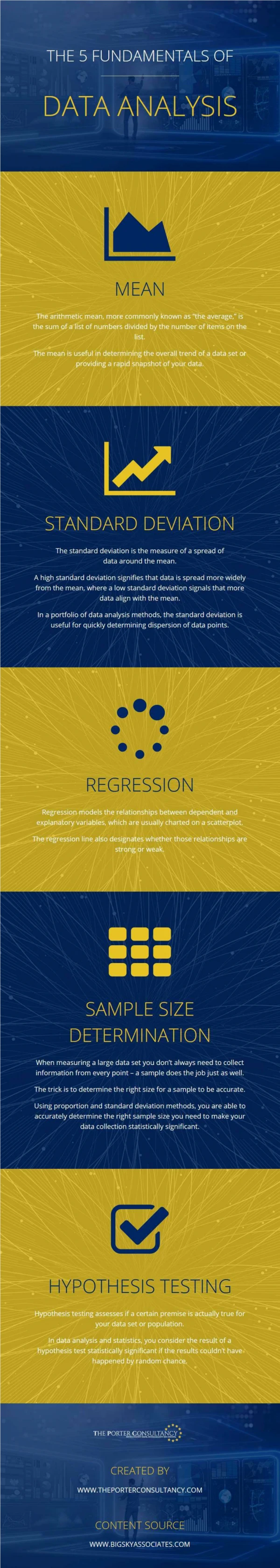
4. What is the statistics ? Definition of Statistics: • A collection of quantitative data pertaining to a subject or group. Examples are blood pressure statistics etc. • The science that deals with the collection, tabulation, analysis, interpretation, and presentation of quantitative data

5. What is the statistics ? Two phases of statistics: • Descriptive Statistics: • Describes the characteristics of a product or process using information collected on it. • Inferential Statistics (Inductive): • Draws conclusions on unknown process parameters based on information contained in a sample. • Uses probability

6. Probability • When we cannot rely on the assumption that all sample points are equally likely, we have to determine the probability of an event experimentally. We perform a large number of experiments N and count how often each of the sample points is obtained. The ratio of the number of occurrences of a certain sample point to the total number of experiments is called the relative frequency.

7. Probability • The probability is then assigned the relative frequency of the occurrence of a sample point in this long series of repetitions of the experiment. This is based on the axiom, called the "law of large numbers", which says that the relative frequency approaches the true (theoretical) probability of the outcome if the experiment is repeated over and over again. How important is the drawing of conclusions based on statistical analysis.

8. Probability where n(E) is the number of times, the event E took place out of a total of N experiments. From this definition we can see that the probability is a number between 0 and 1. When the probability is 1, then we know that a particular outcome is certain.

9. Probability For a discrete random variable definition of probability is intuitive: where n(x)is the number of occurences of the desired value of the random variable x (successes) in N samples (N).

10. Probability • For a continuous random variable, this definition requires the identification of a small range of variation Δx (Δx 0), for which the probability is determined : • For a continuous random variable it is preferable to use the probability density function:

11. Histogram The histogram is the most important graphical tool for exploring the shape of data distributions. And a good way to visualize trends in population data. The more a particular value occurs, the larger the corresponding bar on the histogram.

12. Histogram Constructing a histogram Step 1: Find range of distribution, largest - smallest values Step 2: Choose number of classes, 5 to 20 Step 3: Determine width of classes, one decimal place more than the data, class width = range/number of classes Step 4: Determine class boundaries Step 5: Draw frequency histogram

13. Histogram Number of groups or cells • If number of observations < 100 – 5 to 9 cells • Between 100-500 – 8 to 17 cells • Greater than 500 – 15 to 20 cells

14. Analysis of histogram

15. Analysis of histogram Calculating the average for ungrouped data and for grouped data:

16. Analysis of histogram

17. Measures of dispersion • Range • Standard deviation • Variance

18. Measures of dispersion The range is the simplest and easiest to calculate of the measures of dispersion. R = Xmax - Xmin

19. Measures of dispersion Standard deviation inside the probe:

20. Measures of dispersion For a discrete random variable definition of variation is as follows: when for continous is:

21. Parameters of a distribution • Parameter is a characteristic of a population, i.o.w. it describes a population • Statistic is a characteristic of a sample, used to make inferences on the population parameters that are typically unknown, called an estimator

22. Parameters of a distribution • Population - Set of all items that possess a characteristic of interest • Sample - Subset of a population

23. Parameters of a distribution Expected value (EV) discrete random variable: and for continuous random variable:

24. Random numbers

25. Normal distribution Characteristics of the normal curve: • It is symmetrical -- Half the cases are to one side of the center; the other half is on the other side. • The distribution is single peaked, not bimodal or multi-modal • Also known as the Gaussian distribution

26. Normal distribution Characteristics of the normal curve: • It is symmetrical -- Half the cases are to one side of the center; the other half is on the other side. • The distribution is single peaked, not bimodal or multi-modal • Also known as the Gaussian distribution

27. Normal distribution • Probability density function: • N(μ,σ) • N(0,1) - standard normal distribution is a normal distribution with a mean of 0 and a standard deviation of 1

28. Normal distribution

29. Exponential distribution • Probability density function • Cumulative distribution function for Cumulative distribution function is given by: F(x) = P(-oo, x)

30. Thanks for attention !