Download
1 / 25
250 likes | 446 Views
Fundamentals of Data Analysis Lecture 11 Correlation and regression. Program for today. Basic concepts C orrelation d iagram and correlation table Linear correlation Linear regression The correlation of the multiple variables R egression curves. Basic concepts.

E N D
Fundamentals of Data AnalysisLecture 11Correlation and regression
Program for today • Basic concepts • Correlationdiagram and correlation table • Linearcorrelation • Linearregression • The correlation of the multiple variables • Regressioncurves
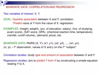
Basic concepts Correlation is defined as the statistical interdependence of measurements of different phenomena, depending on the commonreason or are to each other in a direct causal relationship. Note, however, that the concept of correlation is different from both the causal relationship and the notion of stochastic dependence between random variables.An extreme case is the correlation of co-linear random variables. The correlation is said to be simple or positive when an increase in one variable increases the other. However, when the increase in one variable is accompanied by degrease of second we are dealing with an inverse or negative correlation.
Basic concepts Regression in mathematical statistics is empirically determined the functional relationship between the correlated random variables. Having established that between the studied traits are very weak correlation, proceed to find a regression function that allows you to predict the value of one feature with the assumption that the second characteristic of a defined value. In practice, the most important is the linear regression, corresponding to a linear relationship between the random variables under consideration. Although linear regression is rare in practice, in the form of "pure", but is a convenient tool for obtaining approximate relationships.
Basic concepts • For more complex interdependencies non-linear regression is used, for example a squareregression. • Two models of the data are distinguished: • I-st model , in which the values of the random variable is known (well defined) • II-nd model , in which the random variable is random or vitiated by an error.
Correlationtable and correlation diagram If we have the general population, in which there are two measurable characteristics of X and Y, and they are random variables, and if certain parameters for two-dimensional variable (X, Y) distribution are unknown, this raises the problem of determination of their estimates based on the random sample n pairs of numbers (xi, yi). Treating xi and yi as the coordinates of the point on the plane, a sample can be represented graphically in a correlation diagram.
Correlationtable and correlation diagram To make the table should be for each of the features to build series of distribution, calculating the interval: Rx = xmax - xmin Ry = ymax - ymin then on the basis of the sample size n we take the appropriate number of classes kand calculate the length of the class: dx = Rx / k dy = Ry / k As the lower limit of the first class of variable we accept value slightly lower than the minimum value, and as the upper limit of the last class the value of a little more than the maximum value.
Linearcorrelation The strength of the interdependence of two variables can be expressed numerically by many measures, but the most popular of these is the Pearson correlation coefficient: where the covariance is described in relationship: Estimator of the correlation coefficientrbetween the two test featuresX i Y in the population is the correlation coefficient of the sample, calculated on the basis ofnpairs(xi, yi) of resultswiththeaid of equation:
Linearcorrelation Factor called the coefficient of determination r,with (n-1) degrees of freedom, can be the estimator of correlation.
Linearcorrelation The correlation coefficient takes values between [-1;1]. Coefficient refers to the strength of the relationship. The closer to zero is the weaker relationship them closer to 1 or -1, the stronger. The value of 1 indicates a perfect linear relationship. Sign of the correlation coefficient refers to the direction of union "+" indicates a positive relationship, ie an increase (decrease) in value of one trait will increase (decrease) in the other. "-" Negative direction, ie an increase (decrease) in the value of features results in a decrease (increase) on the other.
Linearcorrelation • Assume the following assessment of the strength of correlation(keeping in mind the appropriate sample size): • below 0.1 - negligible • from 0.1 to 0,3 - weak • from 0.3 to 0.5 - mean • from 0.5 to 0.7 - high • from 0.7 to 0.9 – very high • above 0.9 - almostfull. • Thisscaleisarbitrary.
Correlationtable and correlation diagram Example N = 50measurements of cast dimensionswas made, results areshownin Table. At the 95% confidence level to verify the hypothesis that there is a correlation between the dimensions of the castings.
Correlationtable and correlation diagram Example We calculatethegaps: Rx = 44.5 - 31.1 = 13.4 and Ry = 6.6 - 3.4 = 3.2 As the number of measurements n = 50 we take the number of classes k equal to 7. Thus, the length of the classes are equal: for characteristics of X (dimension): dx = Rx / k = 13.4 / 7 2 and for characteristicsof Y : dy= 3.2 / 7 0.5. As the lower limit for characteristics of X we assume x = 31.0 and for characteristics of Y valuey = 3.25. Thus we get correlation table which is shown in Table
Correlationtable and correlation diagram Example Meanvalues for x = 37.273 and for y = 5.19 and the standard deviationsarerespectively 8.5136 and 0.4544, thus
Linearregression The general populationis given, in which the characteristics (X, Y) have a two-dimensional distribution. Regression straight line of second type for characteristics of Yversus the characteristics of X aregiven by the equation : where: is called the coefficient of a linear regression of characteristics of Y on X, and is the coefficient of the offset.
The correlation of the multiple variables • In the case of correlation of more than two variables the following additional terms should be defined: • Simple correlation (total) is the correlation between the two variables (without taking into account other variables). • Partial correlation is correlation between the two variables when other variables are held constant. • Multiple correlation is a correlation between the number of connected variables, which change simultaneously.
Regressioncurves Regression curves have the general form of the equation: y = a + b1x1 + b2x2+ ... wherebiis the partial regression coefficient of the i-th order.
Regressioncurves Surface chart