Download
1 / 34
360 likes | 523 Views
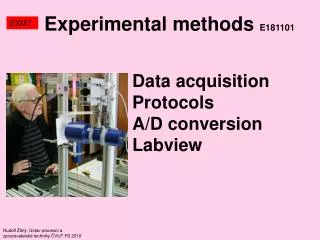
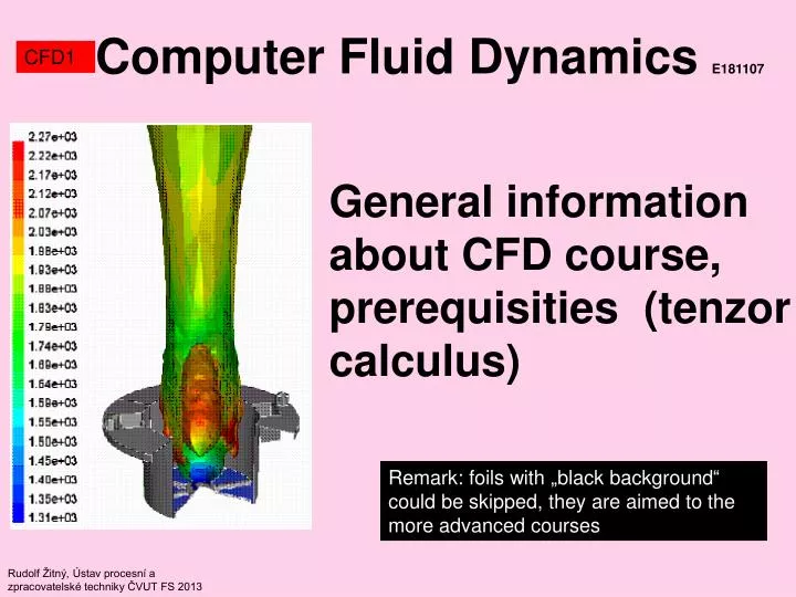
Computer Fluid Dynamics E181107. CFD1. General information about CFD course, prerequisities (tenzor calculus). Remark : fo i l s with „ black background “ could be skipped, they are aimed to the more advanced courses. Rudolf Žitný, Ústav procesní a zpracovatelské techniky ČVUT FS 2013.

E N D
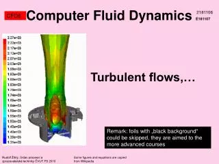
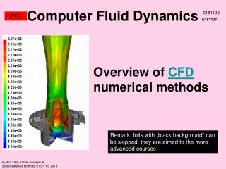
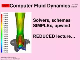
ComputerFluid DynamicsE181107 CFD1 General information about CFD course,prerequisities (tenzor calculus) Remark: foils with „black background“ could be skipped, they are aimed to the more advanced courses Rudolf Žitný, Ústav procesní a zpracovatelské techniky ČVUT FS 2013
Comp.Fluid Dynamics1811072+2 (Lectures+Tutorials), Exam, 4 credits CFD1 Room 304, first lecture 2.10.2014, 9:00-10:45 • LecturesProf.Ing.Rudolf Žitný, CSc. • Tutorialsing.Karel Petera, PhD. • Evaluation excellent very good good satisfactory sufficient failed Summary: Lectures are oriented upon fundamentals of CFD and first of all to control volume methods (application using Fluent) 1. Applications. Aerodynamics. Drag coefficient. Hydraulic systems, Turbomachinery. Chemical engineering reactors, combustion. 2. Implementation CFD in standard software packages Fluent Ansys Gambit. Problem classification: compressible/incompressible. Types of PDE (hyperbolic, eliptic, parabolic) - examples. 3.Weighted residual Methods (steady state methods, transport equations). Finite differences, finite element, control volume and meshless methods. 4. Mathematical and physical requirements of good numerical methods: stability, boundedness, transportiveness. Order of accuracy. Stability analysis of selected schemes. 5. Balancing (mass, momentum, energy). Fluid element and fluid particle. Transport equations. 6. Navier Stokes equations. Turbulence. Transition laminar-turbulent. RANS models: gradient diffusion (Boussinesque). Prandtl, Spalart Alamaras, k-epsilon, RNG, RSM. LES, DNS. 7. Navier Stokes equations solvers. Problems: checkerboard pattern. Control volume methods: SIMPLE, and related techniques for solution of pressure linked equations. Approximation of convective terms (upwind, QUICK). Techniques implemented in Fluent. 8. Applications: Combustion (PDF models), multiphase flows.
CFD KOS CFD1 For more information about the CFD course look at my web pages http://users.fs.cvut.cz/rudolf.zitny/
CFD 2014/2015 CFD1
Jméno DUPS LITERATURE CFD1 • Books: Versteeg H.K., Malalasekera W.:An introduction to CFD, Prentice Hall,1995 Date A.W.:Introduction to CFD. Cambridge Univ.Press, 2005 Anderson J.: CFD the basics and applications, McGraw Hill 1995 Database of scientific articles: You (students of CTU) have direct access to full texts of thousands of papers, available at knihovny.cvut.cz
DATABASE selection CFD1 You can find out qualification of your teacher (the things he is really doing and what he knows) The most important journals for technology (full texts if pdf format)
SCIENCE DIRECT CFD1 Specify topic by keywords (in a similar way like in google) Title of paper is usually sufficient guide for selection.
CFD Applications selected papers from Science Direct CFD1 • Aerodynamics. Keywords “Drag coefficient CFD” (126 matches 2011 , 6464 2012, 7526 2013) Keywords:“Racing car” (87 matches 2011), October 2013 35 articles for: (Drag coefficient CFD) and (Racing car) LES modelling
CFD Applications selected papers from Science Direct CFD1 • Hydraulic systems (fuel pumps, injectors) Keyword “Automotive magnetorheological brake design” gives 36 matches (2010), 51 matches (2011,October). 63 matches (2012,October), 74 (2013) Example
CFD Applications selected papers from Science Direct CFD1 • Turbomachinery (gas turbines, turbocompressors) • Chemical engineering (reactors, combustion. Elsevier Direct, keywords “CFD combustion engine” 1620 papers. “CFD combustion engine spray injection droplets emission zone” 162 papers (2010), 262 articles (2011 October), 364 (October 2013). Examples of matches: LES, non-premix, mixture fraction, Smagorinski subgrid scale turbulence model, laminar flamelets. These topics will be discussed in more details in this course. . kinetic mechanism for iso-octane oxidation including 38 species and 69 elementary reactions was used for the chemistry simulation, which could predict satisfactorily ignition timing, burn rate and the emissions of HC, CO and NOx for HCCI engine (Homogeneous Charge and Compression Ignition) Keywords “two-zone combustion model piston engine” 2100 matches (October 2012), 2,385 (October 2013)
CFD Applications selected papers from Science Direct CFD1 • Environmental AGCM (atmospheric Global Circulation) finite differences and spectral methods, mesh 100 x 100 km, p (surface), 18 vertical layers for horizontal velocities, T, cH2O,CH4,CO2, radiation modules (short wave-solar, long wave – terrestrial), model of clouds. AGCM must be combined with OGCM (oceanic, typically 20 vertical layers). FD models have problems with converging grid at poles - this is avoided by spectral methods. IPCC Intergovernmental Panel Climate Changes established by WMO World Meteorological Association. • Biomechanics, blood flow in arteries (structural + fluid problem)
CFD Applications selected papers from Science Direct CFD1 • Sport Benneton F1
CFD Commertial software CFD1 Tutorials: ANSYS FLUENT Bailey
CFD ANSYS Fluent (CVM), CFX, Polyflow (FEM) CFD1 Single and Multiphase flows Heat transfer & radiation Remark: CFX is in fact CVM but using FE technology (isoparametric shape functions in finite elements) CFX(FEM) ~ Fluent FLUENT = Control Volume Method Incompressible/compressible Laminar/Turbulent flows POLYFLOW = Finite Element Method Incompressible flows Laminar flows Viscoelastic fluids(polymers, rubbers…) Differential models Oldroyd type (Maxwell, Oldroyd B, Metzner White), PTT, Leonov (structural tensors) Integral models Newtonian fluids(air, water, oils…) Turbulence models RANS (Reynolds averaging) RSM (Reynolds stress)
Prerequisities: Tensors CFD1 Bailey
Prerequisities: Tensors CFD1 CFD operates with the following properties of fluids (determining state at point x,y,z): ScalarsT (temperature), p(pressure), (density), h(enthalpy),cA (concentration),k(kinetic energy) Vectors(velocity), (forces), (gradient of scalar) Tensors(stress), (rate of deformation), (gradient of vector) Scalars are determined by 1 number. Vectors are determined by 3 numbers Tensors are determined by 9 numbers Scalars, vectors and tensors are independent of coordinate systems (they are objective properties). However, components of vectors and tensors depend upon the coordinate system. Rotation of axis has no effect upon vector (its magnitude and arrow direction), but coordinates of the vector are changed (coordinates ui are projections to coordinate axis).
Rotation of cartesian coordinate system 2 2’ a2 a’2 1’ a’1 1 a1 CFD1 Three components of a vector represent complete description (length of an arrow and its directions), but these components depend upon the choice of coordinate system. Rotation of axis of a cartesian coordinate system is represented by transformation of the vector coordinates by the matrix product Rotation matrix (Rij is cosine of angle between axis i’ and j’)
Rotation of cartesian coordinate system 2 2’ 1’ CFD1 Example: Rotation only along the axis 3 by the angle (positive for counter-clockwise direction) Properties of goniometric functions therefore the rotation matrix is orthogonal and can be inverted just only by simple transposition (overturning along the main diagonal). Proof: 1
Stresses describe complete stress state at a point x,y,z y y y s s s xy yy zy s x x s x s s yx xx s yz xz s zx zz z z z CFD1 Index of plane index of force component (cross section) (force acting upon the cross section i)
Tensor rotation of cartesian coordinate system CFD1 Later on we shall use another tensors of the second order describing kinematics of deformation (deformation tensors, rate of deformation,…) Nine components of a tensor represent complete description of state (e.g. distribution of stresses at a point), but these components depend upon the choice of coordinate system, the same situation like with vectors. The transformation of components corresponding to the rotation of the cartesian coordinate system is given by the matrix product where the rotation matrix [[R]] is the same as previously
Special tensors CFD1 Kronecker delta (unit tensor) Levi Civita tensor is antisymmetric unit tensor of the third order (with 3 indices) In term of epsilon tensor vector product will be defined
Scalar product y n f x z CFD1 Scalar product (operator ) of two vectors is a scalar aibiis abbreviated Einstein notation (repeated indices are summing indices) Scalar product can be applied also between tensors or between vector and tensor i-is summation (dummy) index, while j-is free index This case explains how it is possible to calculate internal stresses acting at an arbitrary cross section (determined by outer normal vector n) knowing the stress tensor.
Scalar product CFD1 Derive dot product of delta tensor! Define double dot product!
Vector product CFD1 Scalar product (operator ) of two vectors is a scalar. Vector product (operator x) of two vectors is a vector. For example
Vector product Moment of force (torque) CFD 1 Examples of applications Coriolis force application: Coriolis flowmeter
Differential operator CFD1 GRADIENT Symbolic operator represents a vector of first derivatives with respect x,y,z. applied to scalar is a vector (gradient of scalar) applied to vector is a tensor (for example gradient of velocity is a tensor)
Differential operator CFD1 DIVERGENCY Scalar product represents intensity of source/sink of a vector quantity at a point i-dummy index, result is a scalar Scalar product can be applied also to a tensor giving a vector (e.g. source/sink of momentum in the direction x,y,z)
Differential operator CFD1 DIVERGENCY of stress tensor (special case with only one non zero component xx ) x
Laplace operator 2 CFD1 Scalar product =2 is the operator of second derivatives (when applied to scalar it gives a scalar, applied to a vector gives a vector,…). Laplace operator is divergence of a gradient (gradient temperature, gradient of velocity…) i-dummy index Laplace operator describes diffusion processes, dispersion of temperature, concentration, effects of viscous forces.
Laplace operator 2 MHMT1 Positive value of 2T tries to enhance the decreasing part Negative value of 2T tries to suppress the peak of the temperature profile
Symbolic indicial notation CFD1 General procedure how to rewrite symbolic formula to index notation • Replace each arrow by an empty place for index • Replace each vector operator by - • Replace each dot by a pair of dummy indices in the first free position left and right • Write free indices into remaining positions Practice examples!!
Orthogonal coordinates x2 (x1 x2 x3) (r,,z) r x1 CFD1 Previous formula hold only in a cartesian coordinate systems Cylindrical and spherical systems require transformations where Using this it is possible to express the same derivatives in different coordinate systems, for example
Orthogonal coordinates x2 (x1 x2 x3) (r,,z) r x1 CFD1 Transformation of unit vectors Example: gradient of temperature can written in any of the following ways follows from transformation of unit vectors follows from transformation of derivatives (previous slide)
Integral theorems CFD1 Gauss Green (generalised per partes integration)