Download
1 / 54
550 likes | 740 Views
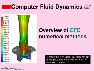
Computer Fluid Dynamics E181107. 2181106. CFD2. Overview of CFD numerical methods. Remark : fo i l s with „ black background “ can be skipped, they are aimed to the more advanced courses. Rudolf Žitný, Ústav procesní a zpracovatelské techniky ČVUT FS 201 3. CFD and PDE. CFD 2.

E N D
ComputerFluid DynamicsE181107 2181106 CFD2 Overview of CFD numerical methods Remark: foils with „black background“ can be skipped, they are aimed to the more advanced courses Rudolf Žitný, Ústav procesní a zpracovatelské techniky ČVUT FS 2013
CFD and PDE CFD2 • CFD problems are described by transport partial differential equations (PDE) of the second order (with second order derivatives). These equations describe transport of mass, species, momentum, or thermal energy. Result are temperature, velocities, concentrations etc. as a function of x,y,z and time t • PDE of second order are classified according to signs of coefficients at highest derivatives of dependent variable (for more details, see next slides): • Hyperbolic equations (evolution, typical for description of waves, finite speed of information transfer) • Parabolic equations(evolution problems, information is only in the direction of evolution variable t - usually time but it could be also distance from the beginning of an evolving boundary layer) • Eliptic equations(typical for stationary problems, infinite speed of information transfer) Examples: supersonic flow around a plane, flow in a Laval nozzle, pulsation of gases at exhaust or intake pipes convection by velocity c Examples: evolution of boundary layer (in this case t-represents spatial coordinate in the direction of flow and x is coordinate perpendicular to the surface of body) Examples: subsonic flows around bodies (spheres, cylinders), flow of incompressible liquids
CFD and PDE CFD2 Why is it important to distinguish types of PDE? Because different methods are suitable for different types (e.g. central differencing in elliptical region and time marching schemes in hyperbolic or parabolic regions)
Characteristics (1/3) CFD2 f can be function of x,y, and first derivatives. x(),y()-parametrically defined curve, where first derivatives p(),q() are specified y x
Characteristics (2/3) CFD2 Right hand side is fully determined by prescribed first derivatives (by boundary conditions) along selected curve Proof!!!
Characteristics (3/3) CFD2 Is the solution of quadratic equation correct? Check signs.
t Value at point x,t is determined only by conditions at red boundary Domain of dependence x Characteristics CFD2 Wave equation - hyperbolic There can be discontinuity across the characteristic lines)
y x PDE type - example CFD2 One and the same equation can be in some region elliptic, in other hyperbolic (for example regions of subsonic and supersonic flow, separated by a shock wave). An example is Prandl-Glauert equation describing steady, inviscid, compressible and isentropic (adiabatic) flow of ideal fluid around a slender body (e.g. airfoil) Function (x,y) is velocity potential, M is Mach number (ratio of velocity of fluid and speed of sound). For M<0 (subsonic flow region) the equation is elliptic, for M>1 (supersonic flow) the equation is hyperbolic. See wikipedia. Another example: Laval nozzle
PDE type – example PWV CFD2 Pulse Wave Velocity in elastic pipe (latex tube, arteries) Model-hyperbolic equations Experiment-cross correlation technique using high speed cameras Macková, H. - Chlup, H. - Žitný, R.: Numerical model for verification of constitutive laws of blood vessel wall. Journal of Biomechanical Science and Engineering. 2007, vol. 2, no. 2/1, p. s66.
PDE type – example WH CFD2 Water Hammer experiment with elastic pipe (latex tube, artificial artery) Model-hyperbolic equations Experiment-cross correlation technique using high speed cameras Pressure sensors
Hyperbolic equations WH CFD2 Flows in a pipe. Time dependent cross section A(t,x), or time dependent mean velocity v(t,x). Compressible fluid or elastic pipe. Relationship between volume and pressure is characterised by modulus of elasticity K [Pa] related to speed of sound a Problem is to predict pressure and flowrate courses along the pipeline p(t,x), v(t,x). Basic equations: continuity and momentum balance (Bernoulli). In simplified form neglected convective term. f-is friction factor Speed of sound Velocity v(t,x) can be eliminated by neglecting friction, giving
Hyperbolic equations WH CFD2 How to derive equations of characteristics multiply by and add both equations
C x2=-at x1=at h/a B A h Method of characteristic CFD2 Integration of PDE along characteristic lines C p=p0 B A v(t)
Pressure profiles n=301 n=101 time (0-3 s) Method of characteristic CFD2 Pipe L=1m, D=0.01 m, speed of sound a=1 m/s, inlet pressure 2 kPa (steady velocity v=0.6325 m/s). l=1;d=0.01;rho=1000;f=0.1;a=1;p0=2e3; v0=(p0*2*d/(l*rho*f))^0.5 n=101;h=l/(n-1);v(1:n)=v0;p(1)=p0; for i=2:n p(i)=p(i-1)-f*rho*v0^2*h/(2*d); end dt=h/a;tmax=3;itmax=tmax/dt;fhr=f*h/(2*a*d); for it=1:itmax t=it*dt; for i=2:n-1 pa=p(i-1);pb=p(i+1);va=v(i-1);vb=v(i+1); pc(i)=a/2*((pa+pb)/a+rho*(va-vb)+fhr*(vb*abs(vb)-va*abs(va))); vc(i)=0.5*((pa-pb)/(rho*a)+va+vb-fhr*(vb*abs(vb)+va*abs(va))); end pc(1)=p0; vb=v(2);pb=p(2); vc(1)=vb+(pc(1)-pb)/(a*rho)-fhr*vb*abs(vb); vc(n)=v0*valve(t); va=v(n-1);pa=p(n-1); pc(n)=pa-rho*a*(vc(n)-va)+f*h*rho/(2*d)*va*abs(va); vres(it,1:n)=vc(1:n); pres(it,1:n)=pc(1:n); p=pc;v=vc; end pmax=max(max(pres))/p0 x=linspace(0,1,n); time=linspace(0,tmax,itmax); contourf(x,time,pres,30)
Le Method of characteristic CFD2 Incorrect boundary condition at exit (elastic and rigid tube connection) D C A e Bernoulli at an elastic tube Bernoulli at a rigid tube
function vrel=pump(t) vrel=0.5*sin(3*t); n=401,Le=2, pmax=803 n=401,Le=1, pmax=709 n=401,Le=0, pmax=669 n=401,Le=0.1, pmax=669 n=401,Le=0.5, pmax=669 Method of characteristic CFD2 Classical numerical methods (Lax Wendroff), require at least slightly flexible connected pipe. MOC seems to be working with a rigid pipe too?
NUMERICAL METHODS CFD2 The following slides are an attempt to overview frequently used numerical methods in CFD. It seems to me, that all these methods can be classified as specific cases of Weighted Residual Methods. Schiele
MWR methods of weighted residuals CFD2 Principles of Weighted Residual Methods will be demonstrated for a typical transport equation (steady state) – transport of matter, momentum or energy Convective transport Dispersion (diffusion) Inner sources Numerical solution (x,y,z) is only an approximation and the previous equation will not be satisfied exactly, therefore the right hand side will be different from zero res(x,y,z) is a RESIDUAL of differential equation. A good approximation should exhibit the smallest residuals as possible, or zero weighted residuals wi are selected weighting functions, and V is the whole analyzed region.
Approximation – base CFD2 Approximation is selected as linear combination of BASE functions Nj(x,y,z) Substituting into weighted residuals we obtain system of algebraic equations for coefficients I (N-equations for N-selected weight functions wi)
xi xi xi Weighting functions CFD2 • Weighting functions can be suggested more or less arbitrarily in advance and independently of calculated solution. However there is always a systematic classification and families of weighting functions. Majority of numerical methods can be considered as MWR corresponding to different classes of weighting functions • Spectral methods (analytical wi(x)) • Finite element methods (Galerkin – continuous weighting function) • Control volume methods (discontinuous but finite weighting function) • Collocation methods (zero residuals at nodal points, infinite delta functions) (Boundary element methods) (or Finite Volume methods) (Finite Differences)
SPECTRALMETHOD ORTHOGONAL FUNCTIONS CFD2 • General characteristics • Analytical approximation (analytical base functions) • Very effective and fast (when using Fast Fourier Transform) • Not very suitable for complex geometries (best case are rectangular regions)
SPECTRALMETHOD ORTHOGONAL POLYNOMIALS CFD2 Weight functions and base functions are selected as ORTHOGONAL functions (for example orthogonal polynomials) Pj(x). Orthogonality in the interval x (a,b) means In words: scalar product of different orthogonal functions is always zero.
WHY ORTHOGONAL? CFD2 Why not to use the simplest polynomials 1,x,x2,x3,…? Anyway, orthogonal polynomials are nothing else than a linear combination of these terms? The reason is that for example the polynomials x8 and x9 look similar and are almost linearly dependent (it is difficult to see the difference by eyes if x8 and x9 are properly normalised). Weight functions and base functions should be as different (linearly independent) as possible. See different shapes of orthogonal polynomial on the next slide. Remark: May be you know, that linear polynomial regression fails for polynomials of degree 7 and higher. The reason are round-off errors and impossibility to resolve coefficients at higher order polynomial terms (using arithmetic with finite number of digits). You can perform linear regression with orthogonal polynomials of any degree without any problem. There is other reason. Given a function T(x) it is quite easy to calculate coefficients of linear combination without necessity to solve a system of algebraic equations: Proof!!!
Orthogonal polynomials CFD2 HERMITE polynomial TSCHEBYSHEF I. polynomial
SPECTRALMETHOD FOURIER EXPANSION CFD2 Goniometric functions (sin, cos) are orthogonal in interval (-,). Orthogonality of. Pn(x)=cos nx follows from for m=n, otherwise 0 Proof!!! In a similar way the orthogonality of sin nx can be derived. From the Euler’s formula follows orthogonality of i-imaginary unit Linear combination of Pj(x) is called Fourier’s expansion The transformation T(x) to Tj for j=0,1,2,…, is called Fourier transform and its discrete form is DFT T(x1), T(x2),…. T(xN) to T1,T2,…TN . DFT can be realized by FFT (Fast Fourier Transform) very effectively.
SPECTRALMETHOD EXAMPLE CFD2 Poisson’s equation (elliptic). This equation describes for example temperature in solids with heat sources, Electric field, Velocity potential (inviscid flows). Fourier expansion of two variables x,y (i-imaginary unit, not an index) Substituting into PDE Evaluated Fourier coefficients of solution • Technical realization • Use FFT routine for calculation fjk • Evaluate Tjk • T(x,y) by inverse FFT
FINITE ELEMENT method CFD2 • General characteristics • Continuous (but not smooth) base as well as weighting functions • Suitable for complicated geometries and structural problems • Combination of fluid and structures (solid-fluid interaction)
y 3 6 5 1 2 x 4 FINITE ELEMENT method CFD2 Base functions Ni(x), Ni(x,y) or Ni(x,y,z) and corresponding weight functions are defined in each finite element (section, triangle, cube) separately as a polynomial (linear, quadratic,…). Continuity of base functions is assured by connectivity at nodes. Nodes xj are usually at perimeter of elements and are shared by neighbours. Base function Ni (identical with weight function wi) is associated with node xi and must fulfill the requirement: (base function is 1 in associated node, and 0 at all other nodes) In CFD (2D flow) velocities are approximated by quadratic polynomial (6 coefficients, therefore 6 nodes ) and pressures by linear polynomial (3 coefficients and nodes ). Blue nodes are prescribed at boundary. Verify number of coeffs.!
FINITE ELEMENT example CFD2 Poisson’s equation Derive Green’s theorem! MWR and application of Green’s theorem Base functions are identical with weight function (Galerkin’s method) wi(x)=Ni(x) Resulting system of linear algebraic equations for Ti
BOUNDARY element method CFD2 • General characteristics • Analytical (therefore continuous) weighting functions. Method evolved from method of singular integrals (BEM makes use analytical weight functions with singularities, so called fundamental solutions). • Suitable for complicated geometries (potential flow around cars, airplanes… ) • Meshing must be done only at boundary. No problems with boundaries at infinity. • Not so advantageous for nonlinear problem. Introductory course on BEM including Fortran source codes is freely available in pdf ( Whye-Teong Ang2007)
BOUNDARY element example CFD2 Poisson’s equation MWR and application of Green’s theorem twice (second derivatives transferred to w) Green’s theorem! Weight functions are solved as a fundamental solution of adjoined equation Delta function! Singularity: Delta function at a point xi,yi Solution (called Green’s function) is Verify!
BOUNDARY element example CFD2 Substituting w=wi (Green’s function at point i) Solution T at arbitrary point xi,yi is expressed in terms of boundary values At any boundary point must be specified either T or normal derivative of T, not both simultaneously. Γ2 (normal derivative) Γ1 (fixed T) dΓ
Γ2 (normal derivative) Γ1 (fixed T) dΓ BOUNDARY element example CFD2 Values at boundary nodes not specified as boundary conditions must be evaluated from the following system of algebraic equations:
FINITE VOLUME method CFD2 • General characteristic: • Discontinuous weight functions • Structured, unstructured meshes. • Conservation of mass, momentum, energy (unlike FEM). • Only one value is assigned to each cell (velocities, pressures). Will be discussed in more details in this course
TN i TE TP TW i TS FINITE VOLUME example CFD2 Poisson’s equation MWR (Green’s theorem cannot be applied because w(x) is discontinuous) Gauss theorem (instead of Green’s) hy hx
FINITE DIFFERENCESmethod CFD2 • General characteristic: • Substitution derivatives in PDE by finite differences. • Suitable for rectangular geometries Will be discussed in more details in this course
Ti-1 Ti Ti+1 x FINITE DIFFERENCES CFD2 Finite differences methods specify zero residuals in selected nodes (the same requirement as in classical collocation method). However, residuals in nodes are not calculated from a global analytical approximation (e.g. from orthogonal polynomials), but from local approximations in the vicinity of zero residual node. It is very easy technically: Each derivative in PDE is substituted by finite difference evaluated from neighbouring nodal values. Upwind 1st order Central differencing 2st order Central differencing 2st order Verify!
Ti,j+1 Ti+1,j Ti,j Ti-1,j y x Ti,j-1 FINITE DIFFERENCESexample CFD2 Poisson’s equation Eliptic equation – it is necessary to solve a large system of algebraic equations
exact solution FINITE DIFFERENCESexample CFD2 Wave equation (pure convection) Hyperbolic PDE-it is possible to use explicit method Lax Wendroff method tn+1 ? First step – Lax’s schemewith time stept/2 t/2 tn x tn+1/2 xk-1 xk xk+1 Second step – central differences tn+1 t tn x tn+1/2 xk-1 xk xk+1
FINITE DIFFERENCESexample CFD2 Wave equation (pure convection) Stability restriction when using explicit methods CFL=0.1 dt=0.011;c=1;l=1;n=101;dx=l/(n-1); cfl=c*dt/dx for i=1:n x(i)=(i-1)*dx; if x(i)<0.1 t0(i)=0; else t0(i)=1; end end tmax=1.;itm=tmax/dt; for it=1:itm for i=2:n-1 ta(i)=(t0(i-1)+t0(i))/2-cfl*(t0(i)-t0(i-1))/2; end ta(1)=t0(1);ta(n)=t0(n); for i=2:n-1 t(i)=t0(i)-cfl*(ta(i+1)-ta(i)); end t(1)=t0(1);t(n)=t0(n); tres(it,:)=t(:); t0=t; end in this case the PDE is integrated along characteristic CFL=1 CFL=1.1
MESHLESS methods CFD2 • General characteristics • Not available in commercial software packages • Suitable for problems with free boundary • Multiphase problems • Easy remeshing (change of geometry) / in fact no meshing is necessary
MESHLESS methods CFD2 There exist many methods that can be classified as meshless, for example SPH (smoothed particle hydrodynamics),Lattice Boltzman (model od particles), RKP(Reproducing Kernel Particle method, Liu:large deformation Mooney), MLPG (Meshless Local Petrov Galerkin), RBF (Radial basis function, wave equation). All the methods approximate solution by the convolution integrals Recommended literature: Shaofan Li, Wing Kam Liu: Meshfree Particle Method, Springer Berlin 2007 (MONOGRAPhy analyzing most of the mentioned method and applications in mechanics of elastoplastic materials, transient phenomena, fracture mechanics, fluid flowm biological systems, for example red blood cell flow, heart vale dynamics). Summary of Galerkin Petrov integral methods Atluri S.N., Shen S.: The meshless local Petrov Galerkin (MLPG) method, CMES, vol.3, No.1, (2002), pp.11-51. Collocaton method: Shu C., Ding H., Yeo K.S.: Local radial basis function-based differential quadrature method and its application to solve two dimensional incompressible Navier Stokes equations, Comp.Methods Appl.Mech.Engng, 192 (2003), pp.941-954
2 1 N+2 N N+1 MESHLESS methods collocation CFD2 Radial base functions where is simply a distance from node j. Most frequently used radial base functions
2 1 N+2 N N+1 MESHLESS methods EXAMPLE CFD2 Poisson’s equation Boundary conditions Approximation i=1,2,….,N (inner points) i=N+1,N+2,…,n (boundary) For multiquadric radial function
MESHLESS method EXAMPLE RBF CFD2 Result is a system of n-linear algebraic equations that can be solved by any solver. In case of more complicated and nonlinear equations (Navier Stokes equations) the system can be solved for example by the least square optimization method, e.g. Marquardt Levenberg. Few examples of papers available from Science Direct
MESHLESS method EXAMPLE RBF CFD2 This radial base function (TPS) was used in this paper
MESHLESS method EXAMPLE RBF CFD2 Comparison with results obtained by FVM package CFD-ACE
MESHLESS method EXAMPLE RBF CFD2 Local topology: each point is associated with nearest NF points …… This is Hardy multiquadrics radial base function