Download
1 / 44
440 likes | 549 Views
An analysis of the H I component of the Magellanic Bridge. Erik Muller: University of Wollongong Australia Telescope National Facility Supervisors: Bill Zealey (UOW) Lister Staveley-Smith (ATNF). Overview: H I observations of the Magellanic Bridge.

E N D
An analysis of the HI component of the Magellanic Bridge Erik Muller: University of Wollongong Australia Telescope National Facility Supervisors: Bill Zealey (UOW) Lister Staveley-Smith (ATNF)
Overview: HI observations of the Magellanic Bridge • HI Data collection and reduction • Magellanic Bridge HI expanding Shell census • Selection Criteria • Shell formation mechanisms • Statistical tools applied to Bridge HI dataset • Spectral Correlation Function • Power Spectrum • Preliminary results for search of CO in emission. • A quick look at some new HI/Hα features in the Bridge.
The Magellanic System: • Detected in HI (spin-flip transition of Neutral Hydrogen) by Kerr, Hindman & Robinson, 1954 with a 36ft Potts hill (Sydney,Australia) reflector. • Their nearness (SMC ~60kpc, LMC ~50kpc) makes them an excellent laboratory in which to observe physical processes with high spatial resolution • Magellanic system comprises five elements: • Large Magellanic Cloud (LMC) (Kim 1998) • Small Magellanic Cloud (SMC) (Staveley-Smith 1998, Stanimirovic 1999) • The Magellanic Stream (Putman, Gibson, Stanimirovic etc. 1998) • The Leading Arm (Putman 2000) • The Magellanic Bridge (Mathewson & Cleary 1984) • Bridge spans the ~14kpc from western edge of LMC to eastern edge of SMC • Formed through tidal interaction of SMC with LMC (Simulations predict 150-200 Myr old - eg. Gardiner & Noguchi 1996) • Populated by young O-B (>7 Myr), as well as older, stars. (eg. Irwin et al, 1995)
LMC, R~50kpc To the Magellanic Stream The Magellanic Bridge l~14kpc To the Leading Arm SMC, R~60kpc The Magellanic System in HI: Parkes Multibeam data obtained by Putman, M.E. Peak Pixel map, Linear trans. func. Tmax=0.3 MJy/beam
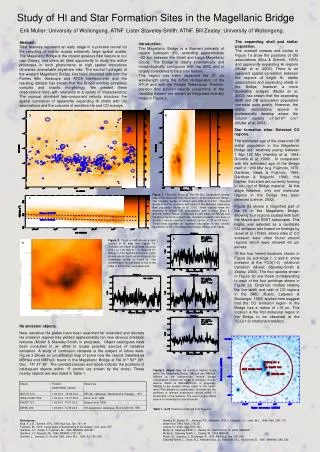
HI Data collection & Reduction: • 144 pointings with ATCA (375m configuration) • ~16 minutes/pointing • Scanning with Parkes multibeam (inner seven beams) • Scanning rate: 1o/min • ATCA Data reduced with MIRIAD • conventional procedures for data flagging and calibration • Parkes data reduced on line with ‘LIVEDATA’ • Bandpass calibrations, velocity corrections • Cube Merging: • Parkes and ATCA data merged post-convolution using IMMERGE (Stanimirovic, PhD, 1999) • Resulting cube: • ~7ox7o region, Vel range~100-350 km/s (Heliocentric) • RMS ~ 15.2 mJy/Beam (eq 1.7x1018 cm2 for each channel) • 98” spatial resolution • ~2x10⁸ M (SMC ~4x10⁸ M)
? Mass of centre region=72x106M (2 x 4.7)kpc cylinder ρ=0.2 atm cm-3 (2 x 4.7 x 5)kpc slab ρ=0.06 atm cm-3 Right Ascension-Declination Velocity-Declination RMS=15.2 mJy/beam (1.7x10¹⁸ atm cm-2) Peak pixel maps of ATCA/Parkes HI datacube Total observed HI Mass=200x106 M 38 km/s [VGSR] 8 km/s [VGSR] Right Ascension-Velocity
Bridge HI Shell census: • Search and census of HI shell features reveal 163 expanding shells within a ~1.9x10⁸ M ofHI. • Strict shell selection criteria must be satisfied • Bridge shells have kinematic ages similar to those found in the SMC, and parameters similar to other galaxies • Distribution of shell centres and positions of OB associations is generally very poor. • Roughly, High HI column density and spatial distribution of OB associations correlate well. Not quite so well at a more detailed level.
Formation mechanisms of HI expanding Shells: • Stellar wind and SNe driven shells (Weaver et al, 1977): • Hot, energetic stars ionise local gas, and blow open an expanding sphere of hot gas. • Study by Rhode et al (1999) on Holmburg II galaxy find that the distribution and brightness of HOII clusters do not support SNe as expansion mechanism. • HVC collisions (Tenorio-Tagle 1987, 1988; Ehlerova & Palous, 1996) • Capable of producing low energy, spherical expanding structures for impacts by low Ek clouds. Rc ~10pc • Difficult/impossible to differentiate from stellar wind formation mechanism. • Distribution of impact sites should be uniform.
Formation mechanisms of HI expanding Shells (cont): • Gamma Ray Bursts (Efremov, Elmegreen & Hodge, 1998; Loeb & Perna, 1998) • Release relatively large amounts of energy (10% of progenitor mass) ~1053 erg • Shells formed from GRB are more energetic for lower radii and more quickly expanding shells. • GBR frequency in a our galaxy ~0.1 Myr –1 (Portegies Zwart, & Spreeuw, 1996). Given the relatively low age and stellar population of the Magellanic we expect this frequency to be significantly reduced. • Ram pressure (Bureau et al, 2001) • ISM Inhomogeneities external to, and impacting on Bridge gas will expand any ‘dimples’ and isolated low-density regions into much larger voids and holes.
Shell selection Criteria • Adapted from Puche et. al. (1992) • A (rough) ring shape in all three projections (RA-Dec, RA-Vel, Dec-Vel), must be present across the velocity range occupied by the shell • Shape is observable across at least three velocity channels (~5km/s) • Ring Must be rim-brightened relative to ambient column density of channel Criteria target rim brightened, expanding spherical structures (not cylindrical or blown out volumes) To reduce subjectivity, criteria must be strictly satisfied! • We assume a stellar wind model (Weaver, 1977)
HI, OB associations and Shells appear to correlate well. HIPeak Pixel map. Size and location of 163 Magellanic Bridge HIexpanding shells. Crosses locate OB associations (Bica et al. 1995) Ret
Comparison of Magellanic Bridge shells to SMC population: • Bridge shells, compared to the SMC population are (on average) • Marginally older, 60% smaller + expand 60% more slowly • Much less energetic: • Mean energy of Bridge: 48.1 (log erg) • Mean energy for SMC: 51.8 (log erg).
MB and SMC HIshell population Decreasing expansion velocity with increasing RA Dynamic age • Generally continuous age distribution • Slight dominance by older shells at higher RA Decreasing shell radius with increasing RA Radius Discontinuity at MB/SMC transition (from strict critera) Expansion Velocity Discontinuity at MB/SMC transition (from strict critera)
Comparison of power law parameters of expanding HIstructures from other surveys • αv is in agreement with other systems • αr is much steeper for the Magellanic Bridge population • Due to a strict selection criteria that manifests as an overall deficiency of small radii shells, and ultimately as an older shell population.
Distribution of OB, shells and HI Black: Left and mean integrated HI in 1.5’x1.5’ region, centred on 198 OB positions. White: Right and entire integrated intensity map, binned into 1.5’2 areas. • OB positions generally correspond regions of higher HI • 50% of OB associations correlate with a Mean HI column density>1.2x10²¹ atm cm-2 • Be wary of selection effects
HI around OB associations • HI ramps almost linearly to centre of OB positions • Excess of HI <80pc of association centre, in disagreement with Grondin & Demers, 1993. • OB associations don’t appear to sweep out a significant hole in the local HI. Diamonds: Mean HI averaged in concentric annuli around OB catalogued positions. Triangles: Mean HI averaged in concentric annuli, offset 90pc (10 pixels) south of OB centres Error bars mark one standard error of the mean, vertical line marks resolution of Parkes observations by Matthewson, Cleary & Murray (1974)
Distribution of OB associations and HIshells • As shown earlier: Visually, OB associations, HI and shell centres appear to correlate reasonably well. • A more quantitative study shows that: • ~50% of shells have one or more OB association within 8’ (140pc) • ~18% of shells have one or more OB associations within 3.5’ (60pc) (mean shell radius) • A study of the variation of the HI column density around OB associations shows in fact and excess within ~80pc of each association (!) • These call into question the commonly used wind/SNe model • Do alternative expansion theories help?
Formation mechanisms of HI expanding Shells: • Stellar wind and SNe driven shells(Weaver et al, 1977 and Chevalier, 1974) • Hot, energetic stars ionise local gas, and blow open an expanding sphere of hot gas. • The most recent burst of star formation 10-25Myr ago (Demers & Battinelli 1998) , C/W mean shell kinematic age ~6Myr • ‘Constant energy input rate is generally invalid’ (Shull, & Saken 1995) • Input from WR and stellar wind at 3~10Myr for coeval and non-coeval associations, mis-estimation of age by up to 40% - lower limit of starburst date by Demers & Battinelli • Bridge Associations & Clusters are very poorly populated, typically N ~ 8 (N increases towards SMC), some Associations & Clusters ‘may be of type later than O-B’ (priv comm. Bica 2002) • Very poor correlation with Bridge Shells (see also Rhode et al. 1999) • A local HIexcess(!) appears co-incident with OB association positions.
Formation mechanisms of HI expanding Shells: • Gamma Ray Bursts(Efremov, Elmegreen & Hodge, 1998; Loeb & Perna, 1998) • Release relatively large amounts of energy (10% of progenitor mass) ~1053 erg • Unlikely to be a significantly frequent occurrence to explain observed shell population for relatively young and poorly-populated stellar component of the Bridge. • GRB Expansion velocities are ~10-2 of velocity for shells of sizes found in the Bridge.
Formation mechanisms of HI expanding Shells: • HVC collisions (Tenorio-Tagle 1987, 1988, Ehlerova & Palous, 1996) • Capable of producing low energy, spherical expanding structures for impacts by low Ek clouds. Rc ~10pc • surface distribution of shells shows a tendency higher HI col. dens. • HVC collisions in tenuous gas may create very asymmetrical and fragmented shells – will not be included in the survey! • An further survey of incomplete shell-like features is necessary before much can be said about the effectiveness of this mechanism. • Ram pressure drag(Bureau et al, 2001) • Mechanism proposed that enlarges ‘dimples’ into deeper holes through interaction of Gas with nearby inhomogeneities • Hole produced this way would not be a complete shell • Holes form this way appear on ‘skin’ of HI mass, MB shells generally deeply embedded.
Statistical tools: • Statistical tools provide a means to • compare populations of similar objects between different systems • Understand and model general trends and behaviours. • Distinguish between sub-populations • Spectral correlation function (SCF): Measures spectral similarity as a function of radial separation • Power spectrum analysis (PS): Measures power as a function of scale, and as a function of velocity range. • Both SCF and PS have been used to infer information about the third spatial dimension.
Spectral Tools 1: • Spectral Correlation function: (Rosolowsky et al. 1999) • Compares two spectra separated by Δr, and makes an estimate of their ‘similarity’ (see later) • A 2D map of mean SCF shows rate of change (or degree of correlation) of SCF with Δr and θ • Has been used to confirm a characteristic length for the scale height of the LMC, by measuring the radius of de-correlation (Padoan et al. 2001) • In this case, SCF shows that MB spectra has a longer de-correlation length in the east-west direction. (Tidal stretching)
Spectral Tools 2: • Spatial power spectrum • Used to show the range of spatial scales present in source • Highlights any process favouring a particular scale. (Eg. Elmegreen, Kim, Staveley-Smith, 2001) • Using velocity averaging, is can be used to show the relative contributions of density and velocity dominated fluctuations. (Lazarian & Pogosyan, 2001) • P-spect shows no characteristic scale in the MB.
Δr Δr Δr Spectral Correlation functionHow it works:
T maps 55 pixels 37 pixels (=2/3 NT) SCF maps
Fits in E-W and N-S directions (central 5 rows/columns) ΣT=1.0x10⁶ K.km/s ΣT=7.5x10⁵ K.km/s ΣT=8.4x10⁵ K.km/s ΣT=9.4x10⁵ K.km/s ΣT=1.0x10⁶ K.km/s ΣT=1.1x10⁶ K.km/s ΣT=1.1x10⁶ K.km/s ΣT=1.1x10⁶ K.km/s • Positive and negative departures from log-log fit after a varying length (~250-380pc ~ 14’-22’ at R=60kpc) • -ve departures seem to exist only for sub images where signal is lower and less well distributed throughout region of interest.
Spatial Power spectrum • Measures the rate of change of power with spatial scale • Works on Fourier inverted image data (edges are rounded by convolution with a small (~30 pixels) gaussian) • Channels with significant signal selected (60 channels) • Filtered to reduce leakage from low spatial frequencies (image convolved with 3x3 unsharp mask, then divided back into FFT data) • Un-observed UV data is masked out. • Power-law fit to remaining dataset (γ) (use IDL poly_fit). • A range of velocity increments are examined to determine the relative contributions of density (thin regime) and velocity (thick regime) fluctuations.
ATCA + Parkes data (+Gaussian rounding) FFT (im2+r2) Spatial Power spectrum cont.
Power law fit for γ – velocity binsize Brightness2 [K2] Transition from thin to thick regime (velocity to density dominated regime) Spatial Power spectrum cont.
General result: • All Power spectra, for all velocity bins are featureless and well fit with by a single power law: • No processes present that lead to a dominant scale (c/w LMC) • More ‘3 dimensional’ than the LMC (Similar to SMC). i.e. no characteristic thickness. • Power spectra steepen for increasing velocity bin size (ΔV~<20km/s) • Transition from ‘thin’ velocity dominated (spectral ΔV ~< integrated ΔV thickness) to thick, density dominated regime. • γ changes from ~-2.90 - ~-3.35, consistent with Kolmogorov Turbulence. (Lazarian & Pogosyan, 2000) • Source of turbulence? • Processes that do not show a scale preference: • Stirring & instabilites from tidal force of LMC and SMC? • Energy deposition into ISM from stellar population?
PS from other systems: • LMC (Elmegreen, Kim & Staveley-Smith, 2001) • much steeper; γ ~<2.7 (Entire velocity range, two linear fits) • LMC spectra turns over at r~100pc • attributed to line-of-sight thickness of LMC. • SMC (Stanimirovic, 1999; Stanimirovic & Lazarian, 2001) • SMC and MB cover same range of γ: • γSMC~ 3.4 at ΔV ~100km/s • γMB~ 3.3 at ΔV ~100km/s • linear (featureless) over entire range of Δv • does not appear to approach a characteristic Δv • Galaxy (Dickey et al. 2001) • Analysed for smaller range of Δv (0-20 km/s) • Inner Galaxy γ ~ -2.5 - -4, consistent with Kolmogorov turbulence. • All systems show steepening of γ with ΔV.
SMC and Galaxy γ with ΔV SMC γ with ΔV. (Stanimirovic & Lazarian, 2001) Galaxy γ with ΔV. (Dickey et al 2001) (N.B. Inverted γ scale, linear ΔV scale)
Star-formation sites in the Magellanic Bridge • The Bridge has a young stellar population • O-B star ages range >7 Myr • SMC has v. low Metallicity (Rubio et al 1993) • ZMB < ZSMC • Bridge formation began ~150-200 Myr ago • Stars are forming in the Bridge • Where are they forming? - Any molecular clouds? • Some recently discovered H2 in the Eastern Magellanic Bridge (Lehner, astro-ph 0206250, 2002) • Any other sites of star formation (Lehner et al 2001, Smoker et al 2000)?
HI Int. Int., 60m contours: (0.4-3.4 +1.9MJy/str) HI Integrated intensity 60m Pointing Offsets by 1 BW (~45”) Candidate 12CO(1-0) emission sites • Local 60m Maximum = dust = surface chemistry. • Local HI Maximum = absorbing layer and raw material
HI and CO spectra suggest the CO emission region is imbedded within an HI cloud: Right: CO Spectra at pointing 1 (solid line and Left axis) overlaid on HI spectra (dotted line and right axis). • 12CO(1-0) detected in emission in the Magellanic Bridge • Star-formation through molecular cloud collapse • Star-formation is a current, active process in the Bridge, even close to SMC. • Stellar population develop in situ, and are not transported from remote location. • Further Evidence of Star-formation in a low-metallicity, tidal structure
Hα structures in the Magellanic Bridge. • One shell has been previously detected in Hα emission that corresponds to an HI shell (Meaburn 1985) • Age calculations from spectroscopic studies disagree with HI shell age estimates by ~10%. (Graham, Meaburn & Bryce (2001) • Contains a UV source (FAUST 392) • Other Hα + HI shells and Hα filaments have since been found • All existing Hα structures in the Bridge are nearby to a FAUST object. (within 2-3”) • Pending further investigations • HI + Hα shells are not significantly different from mean Magellanic Bridge HI shell in terms of radii, expansion velocity, energy etc.
HI: Hα
Summary: • General appearance: • ATCA and Parkes have uncovered chaotic and intricate structure of HI comprising the Magellanic Bridge. • Loops, filaments and clumps observable to smallest scales of 98” (~29pc) • Much of the Bridge is bifurcated into two velocity sheets, converging at ~2hr 30min • Large loop R~1kpc off the northeastern edge of SMC. • Shell survey: • 163 shells found within the Magellanic Bridge • Kinematic age is consistent with that of , shells of the SMC although Magellanic Bridge shells are considerably smaller and less energetic. • Power law distribution of expansion velocity is consistent with HoII and SMC. • Strict selection criteria is insensitive to incomplete and fragmented shells
Summary: • Shells, stars and HI : • Good correlation of HI with OB assocations and Clusters, and also with HI shells (NB. Selection criteria), Poor correlation of OB associations and clusters with expanding shell centres • HI distribution about OB associations and Clusters shows a mean excess at short radii (<80pc), and a decreasing slope with increasing radii • Shell formation: • Shell Energies and spatial distribution do not agree with theories of formation by stellar wind by OB associations and Clusters or by SNe • Frequency of GBRs is too low to be generally applied to Magellanic Bridge shells. • HVCs are capable of producing the observed structures, however, the surface distribution shows preferential distribution (selection effects!), and many shells are found deeply embedded throughout the HIBridge. • Alternatives ??
Summary: • 12CO(1-0) detected in emission for the first time in the Magellanic Bridge • Indication of star formation from molecular cloud collapse (c/w shock triggered star formation) • Star formation within tidal structure and a very low metallicity environment • This presents a unique and opportunity to study star-formation under these conditions at high spatial resolution • Hα filaments throughout the Bridge: • A few are shown to be associated with an expanding HI structure. • All have FAUST objects nearby, the likely source of ionisation.
Summary: • SCF • In general, decorrelation of spectra separated by Δr occurs at ~200-400pc • Estimated thickness of MB is ~5kpc, based on distance measurements for two OB associations separated by ~7’ (Demers & Battinelli, 1998) • Results of SCF are difficult to interpret in the same way for LMC, PS analysis may help. • SCF behaves strangely for datacubes containing low S/N • The line of minimum rate of change of SCF is points almost, but not quite, E-W, towards the SMC and LMC. • Power Spectra • There is no suggestion of a departure from a power law fit to MB spatial power spectra, despite a decorrelation at ~200-400pc found using SCF. (c/w Padoan et al, 2001) • PS shows transition from γ =~-2.9 to γ =-3.35, through thin to thick regime, consistent with Kolmogorov turbulence.