Download
1 / 61
610 likes | 705 Views
Weather/Wind Forecasting and Impact of Surface Conditions on Vertical Profile of Horizontal Winds. William A. Gallus, Jr. Dept. of Geological and Atmospheric Sciences June 7, 2012. How might you forecast the weather (or wind in particular)?. Several Methods can be used:.

E N D
Weather/Wind Forecasting and Impact of Surface Conditions on Vertical Profile of Horizontal Winds William A. Gallus, Jr. Dept. of Geological and Atmospheric Sciences June 7, 2012
Several Methods can be used: • Climatology – just assume winds will behave like they normally do at this location, time of year, and time of day • Statistical – fit observed data using multiple regression, automated neural networks, etc. • Numerical models (Numerical Weather Prediction)
Climatology • Ramp events, very difficult to forecast, can sometimes be best predicted using climatology. • Winds tend to follow seasonal and diurnal trends (reasons to be better understood later) –> near the ground they are strongest during the day and weakest at night. Several hundred meters up, behavior can be opposite. Not fully understood which way they will behave around turbine height of 80 m
Both types of ramps show two peaks during the year. One in May/June corresponds to active period for Low-Level jets and also thunderstorms. Other is in Dec/Jan.
Ramp ups increase sharply to peak in evening (6-9 pm) with minimum in early morning (6-9 am). Ramp downs have peak in early morning (6-9 am) with very pronounced minimum in mid-day hours (9am-3pm).
Statistical Approaches • Can be applied to both observations and model output to look for relationships/correlations. Doesn’t have to make obvious sense. You might find that a prediction of wind 2 hrs from now is most accurate if an equation is used based on phase of the moon, score of recent Cubs game, etc!
Statistical Approaches • Traditionally, in operational forecasting, MOS (Model Output Statistics) is used to refine NWP model output to improve predictions of surface temperature, dew point, and winds. Otherwise, statistical approaches are often avoided by scientists as being “black box”, but they can yield the very best forecasts. These approaches, e.g. MOS, can make use of the other 2: raw NWP output, climatological trends
Numerical Weather Prediction Models • How can you use equations to predict the weather?
Numerical Weather Prediction Models • How can you use equations to predict the weather? • If you have an equation that involves a d/dt, like du/dt = A + B + C, then you can predict the future (you know how the variable, like wind, changes with respect to time)
Can you think of an equation that would allow us to predict future wind?
Can you think of an equation that would allow us to predict future wind? F = ma a = dV/dt So dV/dt = F/m
Numerical Weather Prediction Models • Weather forecasting models are generally built on the Navier-Stokes equations, which come from the basic laws of physics. • These equations are usually discretized, typically via finite differencing, and because they are prognostic equations, they can then predict the future (one time step at a time)
For wind speed prediction, the forecasting equations of interest derive from F=ma. We can re-arrange to write a=F/m, which can yield component equations: Du/Dt = F/m Dv/Dt = F/m Dw/Dt = F/m But, we usually like to forecast at a fixed point (Eulerian framework) instead of in a Lagrangian sense, so we expand the total derivative
We thus have equations that look like: ∂u/∂t = -v▼u - w∂u/∂z = F/m • For horizontal winds (u and v), the forces of importance on the right-hand side include pressure-gradient force, Coriolis force, and Friction. The friction contribution is mostly from the ground. • Pressure gradients are the one force that really “creates” wind. Temperature changes can lead to pressure changes, and thus affect the winds
Coriolis Force (f k x V) just changes the direction of wind (directed to the right in Northern Hemisphere) • Friction ends up being a challenge to treat in the models
Other considerations for NWP • Where do you make your predictions (which kind of horizontal and vertical grid do you use)? w T,u,v T,u,v T T v T,u,v u u w v T T
How exactly do you “discretize” the equations? ut+1 = ut + ▲t – ut (ut, i+1-ut, i-1)/▲x - … or ut+1= ut-1+ 2▲t – (ut, i+1-ut, i)/▲x …
How do you treat atmospheric processes that are too small to be depicted on your grid? Parameterizations are used – and these can vary greatly. Often used for convection, microphysics (cloud physics), turbulence, radiation, land-surface interaction, soil processes….
When we solve equations like these in a numerical forecast model, however, we are really solving for averages (both spatial and temporal)
Reynolds Averaging • Any variable b at any point in space-time can be expressed as a mean and a perturbation: b= b + b’ • The average of perturbations is 0 = b’ • Statistics are stationary over averaging interval
So, if we apply these rules, our equation for u-momentum looks like: ∂u/∂t + ∂u’/∂t = -(u∂u/∂x + u’∂u/∂x +u∂u’/∂x +u’∂u’/∂x) – v….. But averages of single primed terms are 0, so this becomes… ∂u/∂t = -(u∂u/∂x + u’∂u’/∂x) – (v…. Here, the first term is advection of mean wind by mean wind.
Second term is net (mean) contribution from advection of wind fluctuations by the fluctuating part of the wind. These fluctuations are often referred to as “turbulence” but this is not strictly correct – they include ALL fluctuations on scales smaller than the grid volume.
If we look at the sub-grid scale transport terms in more detail, we can use the product rule of differentiation and rearrange to show that • ∂u/∂t = -u∂u/∂x -∂/∂x(u’u’) - u’∂u’/∂x Where the second term is recognizable as “turbulence flux divergence” (or sub-grid) Last term can be re-written and shown to equal zero assuming incompressible continuity
Closure Issue • Our entire set of governing equations then ends up consisting of 7 equations, with 7 first-moment variables (u,v,w,Θ,ρ,p,T – all of these having overbars on them), but we have ended up with 8 second-moment unknowns from the averaging procedure.
If we make more predictive equations for the second moments, we don’t fix the problem, because we then end up with additional terms involving the third moment [like ∂/∂x(u’u’u’) ]. • We cannot close the system by adding equations for the higher-order terms. To obtain a closed system, we have to do something about the higher-order terms.
Obtaining a closed system • We can either ignore higher-order terms • Or…represent them as a function of lower-order variables
First-order closure • For first-order closure, used in almost all forecasting models, we have equations to predict the first-order moments, and we represent higher-order moments as a function of the first-order ones.
Gradient-transfer theory • Most common approach to first-order closure is called gradient-transfer theory. We represent fluxes as proportional to gradients of mean variables: u’b’ = -K ∂b/∂x So, subgrid flux in a given direction is proportional to gradient in that direction, and transport is down-gradient (from high values of b toward low ones)
Also, transport depends on the LOCAL GRADIENT (∂b/∂x) • The K terms can be anisotropic, meaning we could have different values for horizontal versus vertical transport
Specification of Ks • We can use profile methods – specify some function giving realistic distribution of K with height, so that it is small near ground, large in lower half of Planetary Boundary Layer (PBL), and smaller again near top of PBL • Local stability/mixing length – K’s are specified by some functional form so they are small where atmosphere is stable and increase as atmosphere becomes less stable
Mixing Length (cont) • These schemes specify a “mixing length”. A “law of the wall” type approach is used so that l -> 0 at the ground (l=kz) where k=von Karman’s constant (around 0.4). An upper bound is placed on k so that l< l0 of roughly 50-100 m
A widely-recognized deficiency in gradient-transfer theory is that sometimes fluxes do not depend on local gradients. Convective eddies in daytime PBL transport heat across the entire PBL depth (from ground to top), and this transport is related more to bulk PBL properties than local gradients. It is possible to try to include some of these non-local effects.
PBL (Mixed Layer) Growth Definition – layer of the atmosphere having its behavior directly affected by the surface The PBL typically grows deeper during the day as the sun warms the ground, and rapidly collapses at night
Potential temperature is a concept often used to depict the PBL –> θ = T (1000/p)R/cp β=∂θ/∂z zi Z PBL heat The layer with uniform potential temperature is referred to as the mixed layer (or PBL), and its top is usually denoted zi (where “i” stands for “inversion”)
The redistribution of air parcels corresponds to a heat flux. We represent the kinematic heat flux as w’’θ’’, i.e., correlations of turbulent vertical motions with turbulent fluctuations of temperature. • The heat flux warms the temperature and deepens the PBL • A deeper PBL generally means that higher-speed winds from higher levels in the atmosphere are “mixed” down to the region near the surface (and vice-versa… friction-slowed air is mixed upward)
Land use/characteristics impact the PBL • How much friction is a function of the characteristics of the earth’s surface • Lots of trees/hills/tall buildings lead to lots of friction and slowing of flow • Cold water or snow prevents warming and thermals, confining friction to layer right near ground, without much PBL development
Things get really interesting as the sun is getting ready to set • Cooling first happens near the ground, so a stable layer forms there, and this “decouples” the atmosphere from the surface. Friction now has very little impact on the air in the lower atmosphere. Remnant PBL Stable layer
Removal of friction allows the air a short distance above the ground (50-1000 m) to begin accelerating, with speeds increasing and directions veering (clockwise) • Coriolis force leads to an “inertial oscillation” so that winds peak in speed around 1 or 2 am => Low Level Jet
PBL parameterizations in models – example from WRF • Non-local: 1) ACM2 (or Pleim) 2) YSU • Local: 1) MYJ 2) QNSE 3) MYNN2.5 4) MYNN3.0
Biases in 80m wind forecasts using different PBL schemes in WRF model Note: YSU is most different Composites of PBL biases by hour. Each line represents a different PBL scheme; MYJ (Black), MYNN 2.5 (Red), MYNN 3.0 (Blue), Pleim or ACM2 (Green), QNSE (Cyan), and YSU (Magenta).
Differences in predictions of Low-Level Jets from one case using WRF model Observed peak Wind speed as a function of height profile during the LLJ peak on March 24, 2009 at 10pm LST. Black dots represent observations from the 915-mHz wind profiler while each line represents a different PBL scheme; MYJ (Black), MYNN 2.5 (Cyan), MYNN 3.0 (Magenta), Pleim or ACM2 (Red), QNSE (Blue), and YSU (Green).
Three hour averaged diurnal cycle of ramp-up events using the midpoint of the ramp event. Black line is observed ramp-up events. Note the very different behavior of the YSU scheme, and to a lesser extent the Pleim
Example of challenges of creating a good NWP forecast system for Wind Based on M.S. work of Adam Deppe
NWP Model (WRF) was run over these 2 domains/grid spacings Which would you think should give the best forecast and why???
Model domain and location of verification data Figure 2. (Left) The 10 km domain with outline of Pomeroy wind farm (right) where the individual wind turbines are the black dots and the 80 m meteorological tower (observed data location) is the X.
The spread (variety) has increased but not the skill (MAE not reduced) so this is not a good solution
For this domain and cases, the 4 km model domain did not work as well. Ideas why?
Different time initializations lead to lower skill AND higher spread