Download
1 / 51
510 likes | 528 Views
This algorithm utilizes a texture-based approach to extract geographic information from remotely sensed data. It incorporates LiDAR and passive optical imagery, allowing for accurate mapping of various phenomena such as forests, urban features, population density, and vehicle density.

E N D
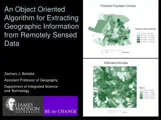
An Object Oriented Algorithm for Extracting Geographic Information from Remotely Sensed Data Zachary J. Bortolot Assistant Professor of Geography Department of Integrated Science and Technology BE the CHANGE
Objective: To create an object oriented algorithm that incorporates the strengths of the texture-based approach
To meet this objective the Blacklight algorithm was created • Three versions exist: • Three band passive optical • Panchromatic passive optical • -Three band passive optical plus LiDAR
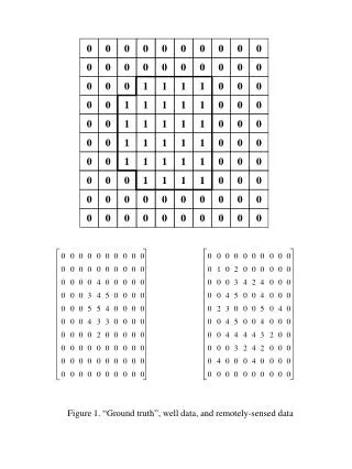
The project setup window for the version that uses LiDAR and passive optical imagery The data in the spreadsheet consists of data on the phenomena you would like to map made on the ground using a GPS unit or through image interpretation. In this case the data are trees / hectare for a forest.
Next, the user uses sliders to identify objects he or she thinks may be related to the attribute of interest.
The sliders work by creating a linear equation based on a series of images created using simple image processing operations. This equation should maximize the response to the object, and minimize the response to the background. If the equation value is greater than 0, a pixel is considered to be part of the object. In this case the equation is:
Once the objects have been initially identified, metrics can be calculated based on the object. For example: The percentage of the plot taken up by objects. The percentage of the object pixels that are core pixels. These metrics are used in a regression equation to predict the measured attribute. = Core pixel Percent core = 12.5%
To improve the prediction accuracy, an optimization procedure is run which adjusts the sliders.
The values image. In this case the number of trees per hectare in the area under the crosshairs is 1810.47. A map showing the phenomena over the whole area of interest. Clicking on a pixel will bring up the estimated value at that location.
Tests Test 1: Mapping forests Test 2: Mapping urban features Test 3: Mapping population density Test 4: Mapping vehicle density
Test 1: Mapping forests Remotely sensed data: 0.5m color infrared orthophotograph Normalized DSM with a 1m resolution, obtained from DATIS II LiDAR data with a 1m point spacing. Reference data: 10 circular plots with a 15 m radius placed in 11 – 16 year old non-intensively managed loblolly pine plantations at the Appomattox-Buckingham State Forest in Central Virginia. The following values were measured: Trees per hectare Biomass
This map was produced by averaging the predicted values in each stand.
This map was produced by segmenting the predicted biomass output from Blacklight using the SARSEG module in PCI Geomatica.
This map was produced by averaging the predicted values in each stand.
This map was produced by segmenting the output from Blacklight using the SARSEG module in PCI Geomatica.
Test 2: Mapping the urban environment Imagery: 1m normal color USDA NAIP data of Morehead, Kentucky from 2004. Reference data: 25 randomly selected 100 x 100m plots in which the following were calculated based on photointerpretation: Percent impervious Percent tree cover Percent grass
The values image. In this case 91.7% of the cell is estimated to contain impervious surfaces.
Test 3: Population density Imagery: 1m normal color USDA NAIP data of Harrisonburg, VA from 2003. Reference data: US Census data from 2000. 20 censusblockswere randomly selected and 50 x 50m areas at the center of each plot were used for processing. Mapping population density would be of use in developing countries with no recent, reliable census data.
This map was produced by averaging the predicted values in each census tract.
This map was produced by segmenting the output from Blacklight using the SARSEG module in PCI Geomatica.
Test 4: Vehicle density Imagery: 6” normal color Virginia Base Map Program data of Harrisonburg, VA from 2006. Reference data: Photointerpreted vehicles per acre
Conclusions The algorithm shows promise in multiple types of analysis Planned improvements: Additional image processing functions Better LiDAR integration Additional object metrics Ability to select metrics based on a stepwise approach