Download
1 / 42
430 likes | 573 Views
1. 11. 1. 1. 1. 1. 1. 1. 1. 1. 2. 2. 3. 3. 1. 4. 4. 5. 1111111111. 3455. 5. 5. 1. 5. 1. 5. An arrangement of lines: A(H). Elements of the arrangement. Vertices – intersection of lines Edges – portions of lines bounded by vertices, except when unbounded at one end

E N D
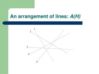
1 11 1 1 1 1 1 1 1 1 2 2 3 3 1 4 4 5 1111111111 3455 5 5 1 5 1 5 An arrangement of lines: A(H)
Elements of the arrangement • Vertices – intersection of lines • Edges – portions of lines bounded by vertices, except when unbounded at one end • Faces – regions bounded by edges and vertices
Counts of the elements • Number of vertices (V) : n(n-1)/2 • Number of edges (E): n^2 (interesting) • Number of faces (F): n^2 – n(n-1)/2 + 1 (follows from the modified Euler formula V-E+F = 1)
Computing an arrangement • We must output a data structure that encapsulates the mutual relationships of the elements (vertices, edges and faces), corresponding to the pictorial representation of an A(H) as in the first slide • EG paper only shows how to traverse A(H)
Sweepline paradigm • The standard sweepline paradigm requires sorting the O(n^2) intersection points • This would require O(n^2 log n) time
Topological sweep • Gets rid of the log n factor, by processing the intersection points without having to sort them !! • It does this at the expense of just O(n) additional space needed by lots of extra book-keeping.
A partial order • We can define the following partial order on elements of the arrangement • An element A isabove element B if A is above B at every vertical line that intersects both A and B • The above relationship is acyclic • The inverse of above is below
Consequences • There exists a unique element in A(H)that is not below any other and a unique element that is not above any other. • These are called respectively the top-most and the bottom-most element • Prove uniqueness from the acyclicity of the above partial order
Cuts • A cut is a sequence of edges (c1, c2, ...,cn), one from each line of A(H), such that for each i (1.. n-1) there is a (unique) face fi such that ci is above fi , and c(i+1) is below fi • c1 is below the top-most face and cn is above the bottom-most face
c1 c2 c3 c4 A cut – pictorially c5
Ordering the cuts • A cut C is is to the left of a cut C' if for eachlinelin A(H), cionlfrom C is to the left of oridentical withcjfrom C' onl • Thus there is a lefmost cut and a rightmost one
Important Fact • In a given cut there exists an i such that ci and c(i+1) have a common right end-point • The so-called topological sweep exploits this to move from the leftmost cut to the rightmost one in a series of elementary moves • In each such move, the topological line moves across such a common right end-point • We demonstrate this on the example arrangement in the next few slides
Sweeping the arrangement The leftmost cut
10th elementary move The rightmost cut
Representing a cut • A cut is represented by an array C[1..n], where each C[i] = ( λi, ρi ,µi), representing respectively the index of the line that defines the left and right end-point of the edge ci and the index of the line on which it lies
From one cut to the next.. • This is done in an elementary step • An elementary step is one in which the topological sweep moves across an intersection defined by ci and c(i+1) for some i in the current cut • Such an i always exists except when the cut is the rightmost one
Implementing an elementary move • An elementary move is implemented with the help of two data structures derived from a cut C – namely the upper horizon tree T+(C) and the lower horizon tree T-(C)
Data Structures for horizon trees • An array HTU[1..n] for the upper horizon tree, where HTL[i] = (λi, µi), where λi (µi ) is the index of the line that defines the left (right) end point of the segment from li that belongs to the upper horizon tree • λi = -1 if segment left-unbounded and µi = 0 if right-unbounded • A similar definition for HTL[1..n]
Example HTU[1..5] HTU[1]= (-1,2) HTU[2]= (-1,5) HTU[3]= (5,4) HTU[4]= (5,0) HTU[5]= (3,0)
Example HTL[1..5] HTL[1]= (-1,0) HTL[2]= (-1,1) HTL[3]= (5,1) HTL[4]= (5,3) HTL[5]= (3,1)
Data Structures for horizon trees • Array M[1..n] stores the index of the line on which ci lies • Array N[1..n] stores the description of a cut; N[i] = (λi, µi), where λi (µi )is the index of the line that defines the left-end (right-end) of ci • N[1..n] can be obtained from HTL[1..n], HTU[1..n] and M[1..n]
Example N[1..5] • M[1..5] = [1,2, 5, 3, 4] (slide 32) • This gives: N[1..5] = [(-1,2), (-1,1), (3,1), (5,4),(5,3)]
Data Structures for horizon trees • Finally, we have a stack I that stores the indices i such that ci and c(i+1) have a common right end-point. • This is obtained from N[1..n] by examining pairs of entries in N[1..n] and checking if µi = µi+1 + 1, for i= 1, .., n-1, and stacking the i for which the above holds
Example I • I=[1,4 …….., for the example N[1..5]
Updating all the other data structures • It is easy to update M[1..n] • N[i] = HTL[M[i]] ∩ HTU[M[i]] • From N[i] we can update the stack I
Analysis • The analysis shows that the cost of traversing the bays associated with a fixed line l is O(n) and hence O(n2) for all n lines.