NUMERICAL DESCRIPTIVE STATISTICS Measures of Variability
270 likes | 501 Views
NUMERICAL DESCRIPTIVE STATISTICS Measures of Variability. Another Description of the Data -- Variability. For Data Set A below, the mean of the 10 observations is 2.60. SET A: 4,2,3,3,2,2,1,4,3,2

NUMERICAL DESCRIPTIVE STATISTICS Measures of Variability
E N D
Presentation Transcript
NUMERICAL DESCRIPTIVE STATISTICS Measures of Variability
Another Description of the Data -- Variability • For Data Set A below, the mean of the 10 observations is 2.60. SET A: 4,2,3,3,2,2,1,4,3,2 • But each of the following two data sets with 10 observations also has a mean of 2.60 SET B: 2,2,2,2,3,3,3,3,3,3 SET C: 0,0,1,1,4,4,4,4,4,4 • Although sets A, B, an C all have the same mean, the “spread” of the data differs from set to set.
Data Set A Data Set B Most “spread” Least “spread” Data Set C The “Spread” of the Data
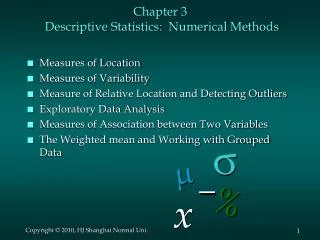
Measures of Variability • Population • Variance 2 • Standard Deviation • Sample • Range • Variance s2 • Standard Deviation s
The Range • When we are talking about a sample, the range is the difference between the highest and lowest observation • In the sample there were some A’s (4’s), and the lowest value in the sample was a D (1) • Sample range = 4 - 1 = 3
Another Approach to Variability • The range only takes into account the two most extreme values • A better approach • Look at the variability of all the data • In some sense find the “average” deviation from the mean • The value of an observation minus the mean can be positive or negative • The plusses and minuses cancel each other out giving an average value of 0 • Need another measure
How to Average OnlyPositive Deviations • MEAN ABSOLUTE DEVIATION (MAD) • Averages the absolute values of these differences • Used in quality control/inventory analyses • But this quantity is hard to work with algebraically and analytically • POPULATION VARIANCE (σ2) • Averages the squares of the differences from the mean
EXAMPLECalculation of σ2 Using the numbers from the population of 2000 GPA’s: 4,2,1,3,3,3,2,… 2
Standard Deviation • But the unit of measurement for σ2 is: • Square Grade Points (???) • What is a square grade point? • To get back to the original units (grade points), take the square root of σ2 • STANDARD DEVIATION () – the square root of the variance, σ2
Calculation of theStandard Deviation (σ) • For the grade point data:
Estimating σ2 • SAMPLE VARIANCE (s2) • Best estimate for is 2 is s2 • s2 is found by using the sample data and using the formula for 2 except:
Calculations for s2 • The data from the sample is: 4,2,3,3,2,2,1,4,3,2
Sample Standard Deviation, s • The best estimate for is denoted: s • It is called the sample standard deviation • s is found by taking the square root of s2
s2 for Grouped Data • For the grade point example • 4 occurs 2 times • 3 occurs 3 times • 2 occurs 4 times • 1 occurs 1 time • To calculate the sample variance, s2, rather than write the term down each time: • Multiply the squared deviations by their class frequencies
Empirical RuleInterpreting s(Mound Shaped Distribution) • If data forms a mound shaped distribution • Within 1s from the mean • Approximately 68% of the measurements • Within 2s from the mean • Approximately 95% of the measurements • Within 3s from the mean • Approximately all of the measurements
Chebychev’s InequalityInterpreting s(Any Distribution) • If data is not mound shaped ( or shape is unknown) • Within 2s from the mean • At least 75% of the measurements • Within 3s from the mean • At least 88.9% of the measurements • Within ks from the mean (k > 1) • At least 1 -1/k2 of the measurements
Coefficient of Variation • Another measure of variability that is frequently used to compare different data sets (even if measured in different units) is the: Coefficient of Variation (CV) CV = (Standard Deviation/Mean) x 100%
Range Approximation for σ • If data is relatively mound-shaped a “good” approximation for s is: σ (range)/4 Sometimes, when one is more certain that the sample range captures the entire population of data statisticians use, σ (range)/6
Using Excel • Suppose population data is in cells A2 to A2001 Population variance (2) = VARP(A2:A2001) Population standard dev. () =STDEVP(A2:A2001) • Suppose sample data is in cells A2 to A11 Sample variance (s2) =VAR(A2:A11) Sample standard dev. (s) =STDEV(A2:A11) • Data Analysis
Check Labels Where data values are stored Check both: Summary Statistics Confidence Level Enter Name of Output Worksheet
Drag to make Column A wider Sample Standard Deviation Sample Variance
Review • Measures of variability for Populations and Samples • Range • Variance • Standard Deviation • Interpretation of standard deviation • Empirical Rule for “mound-shaped” data • Chebychev’s Inequality for “other” data • Excel • Functions • Data Analysis