CHAPTER 3 : DESCRIPTIVE STATISTIC : NUMERICAL MEASURES (STATISTICS)
CHAPTER 3 : DESCRIPTIVE STATISTIC : NUMERICAL MEASURES (STATISTICS). DESCRIPTIVE STATISTICS : NUMERICAL MEASURES (STATISTICS ). 3.1 Measures of Central Tendency Gives the center of a histogram or a frequency distribution curve. 3.1.1 Different measures of central tendency i. Mean

CHAPTER 3 : DESCRIPTIVE STATISTIC : NUMERICAL MEASURES (STATISTICS)
E N D
Presentation Transcript
CHAPTER 3 : DESCRIPTIVE STATISTIC : NUMERICAL MEASURES (STATISTICS)
DESCRIPTIVE STATISTICS : NUMERICAL MEASURES (STATISTICS) 3.1 Measures of Central Tendency • Gives the center of a histogram or a frequency distribution curve. 3.1.1 Different measures of central tendency i. Mean • The mean of a sample is the sum of the measurements divided by the number of measurements in the set. Mean is denoted by Mean = Sum of all values / Number of values • Mean can be obtained as below :- For ungrouped data, mean is defined by,
For grouped data, mean is defined by, Where f = class frequency; x = class mark (mid point) Example 3.1:- The mean sample of CGPA (raw) is Table 3.1
Example 3.2 :- The mean sample for Table 3.2 Table 3.2
ii. Median • Median is the middle value of a set of observations arranged in order of magnitude and normally is devoted by • The median for ungrouped data. - The median depends on the number of observations in the data, . - If is odd, then the median is the th observation of the ordered observations. - If is even, then the median is the arithmetic mean of the th observation and the th observation.
2. The median of grouped data / frequency of distribution. The median of frequency distribution is defined by: where, • = the lower class boundary of the median class; • = the size of the median class interval; • = the sum of frequencies of all classes lower than the median class; and • = the frequency of the median class.
Example 3.3 for ungrouped data :- The median of this data 4, 6, 3, 1, 2, 5, 7, 3 is 3.5. • Rearrange the data in order of magnitude becomes 1,2,3,3,4,5,6,7. As n=8 (even), the median is the mean of the 4th and 5th observations that is 3.5. Example 3.4 for grouped data :- = 3.217 Proof :- Median Table 3.3
iii. Mode • The mode of a set of observations is the observation with the highest frequency and is usually denoted by . Sometimes mode can also be used to describe the qualitative data. • Mode of ungrouped data :- - Defined as the value which occurs most frequent. - The mode has the advantage in that it is easy to calculate and eliminates the effect of extreme values. - However, the mode may not exist and even if it does exit, it may not be unique.
*Note: • If a set of data has 2 measurements with higher frequency, therefore the measurements are assumed as data mode and known as bimodal data. • If a set of data has more than 2 measurements with higher frequency so the data can be assumed as no mode. 2. The mode for grouped data/frequency distribution data. - When data has been grouped in classes and a frequency curve is drawn to fit the data, the mode is the value of corresponding to the maximum point on the curve.
- Determining the mode using formula. where = the lower class boundary of the modal class; = the size of the modal class interval; = the difference between the modal class frequency and the class before it; and = the difference between the modal class frequency and the class after it. *Note: - The class which has the highest frequency is called the modal class.
Example 3.5 for ungrouped data :- The mode for the observations 4,6,3,1,2,5,7,3 is 3. Example 3.6 for grouped data based on table :- Proof :- Table 3.4
3.2 Measure of Dispersion • The measure of dispersion or spread is the degree to which a set of data tends to spread around the average value. • It shows whether data will set is focused around the mean or scattered. • The common measures of dispersion are variance and standard deviation. • The standard deviation actually is the square root of the variance. • The sample variance is denoted by s2 and the sample standard deviation is denoted by s.
3.2.1 Range • The range is the simplest measure of dispersion to calculate. Range = Largest value – Smallest value Example 3.7:- Table 3.5 gives the total areas in square miles of the four western South-Central states the United States. Range = Largest Value – Smallest Value = 267, 277 – 49, 651 = 217, 626 square miles. Table 3.4
3.2.2 Variance • Variance for ungrouped data - The variance of a sample (also known as mean square) for the raw (ungrouped) data isdenoted by s2 and defined by: • Variance for grouped data - The variance for the frequency distribution is defined by:
Example 3.8 for ungrouped data :- Variance for the Students’ CGPA for Data 1 is 0.105. Example 3.9 for grouped data :- The variance for frequency distribution in Table 3.5 is: Table 3.5
3.2.3 Standard Deviation • Standard deviation for ungrouped data :- ii. Standard deviation for grouped data :-
Example 3.10 (Based on example 3.8) for ungrouped data: Example 3.11 (Based on example 3.9) for grouped data:
3.2.4 Rules of Data Dispersion • Chebyshev’s Theorem • At least of the observations in will be in the range of standard deviation from mean, where is the positive number exceed 1. Steps: • Determine the interval • Find value of • Change the value in step 2 to a percent • Write statement: at least the percent of data found in step 3 is in the interval found in step 1 • Example 3.12:- = = = = 0.75 Hence, according to Chebyshev`s Theorem, at least 75% of the value of a data set lie within two standard deviations of the mean.
Empirical Rule - For a data that is normally distributed, at least i. 68% of the observations lie in the interval ii. 95% of the observations lie in the interval iii. 99.7% of the observations lie in the interval