Download
1 / 12
120 likes | 310 Views
Numerical Measures of Variability. Deviations and the Spread of Data. A deviation is the difference between an observation value and the mean of its sample or population distribution. The sum total of all deviations in a sample or population always equals zero.

E N D
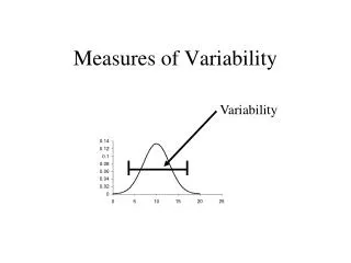
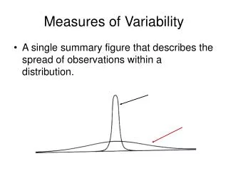
Deviations and the Spread of Data A deviation is the difference between an observation value and the mean of its sample or population distribution. The sum total of all deviations in a sample or population always equals zero. But deviations tell us something more about the sample or population than does a measure of central tendency, such as the mean. The greater the deviations – both positive and negative – the more “spread out” is the data.
Example: Consider the difference between the ages of students in a KKU school bus….. …and the ages of passengers in a typical city bus. Let’s take a sample of the ages of n = 20 passengers (“observations”) in each of the two buses. Note that, even though the spread of ages on the city bus is larger than that of the school bus, we can’t use the total deviations to show this! *Mean = Σtotal/n = Σtotal/20
Returning to the bus example the range R on the two buses is R(KKU) = 24 – 19 = 5 and R(City) = 67 – 2 = 65
To use more of the information in the data set, the Interquartile Range can be used instead. The Interquartile Range is found by ordering the data set as above, eliminating the lowest quarter (25%) of the data set and the highest quarter (25%) of the data set, and then finding the range of the middle half (50%) of the data set.
Mean Absolute Deviation (MAD) In mathematics, a number’s absolute value is that same number, but expressed as a positive number without the minus sign (if it is a negative number). Straight vertical lines denote the absolute value. Absolute value of 3 = |3| = 3 Absolute value of – 3 = |-3| = 3 The Mean Absolute Deviation (MAD) takes the absolute value of each of the sample deviations, and then gets the mean of these values for the sample as a whole.
Just ignore the minus signs! Because there are 7 sample values, the MAD = 32/7 = 4.57
Returning to the School Bus & City Bus Example….. n = 20 passengers MAD = Σ|Deviation|/n = Σ|Deviation|/20 Note that the City Bus’s MAD is much larger than the KKU School Bus’s MAD, just as our intuition would suggest.