Download
1 / 28
300 likes | 579 Views
A reaction-advection-diffusion equation from chaotic chemical mixing. Junping Shi 史峻平 Department of Mathematics College of William and Mary Williamsburg, VA 23187 ,USA. Math 490 Presentation, April 11, 2006,Tuesday. Reference Paper 1: Neufeld, et al, Chaos, Vol 12, 426-438, 2002.

E N D
A reaction-advection-diffusion equation from chaotic chemical mixing Junping Shi史峻平 Department of Mathematics College of William and Mary Williamsburg, VA 23187,USA Math 490 Presentation, April 11, 2006,Tuesday
Reference Paper 1:Neufeld, et al, Chaos, Vol 12, 426-438, 2002
Reference paper 2: Menon, et al, Phys. Rev. E. Vol 71, 066201, 2005
Model • The spatiotemporal dynamics of interacting biological or chemical substances is governed by the system of reaction-advection-diffusion equations: where i=1,2,….n, C_i(x,t) is the concentration of the i-th chemical or biological component, f_i represents the interaction between them. All these species live a an advective flow v(x,t), which is independent of concentration of chemicals. Da, the Damkohler number, characterizes the ratio between the advective and the chemical or biological time scales. Large Da corresponds to slow stirring or equivalently fast chemical reactions and vice versa. The Peclet number, Pe, is a measure of the relative strength of advective and diffusive transport.
Arguments to derive a new equation • At any point in 2-D domain, there is a stable direction where the spatial pattern is squeezed, and there is an unstable direction where the pattern converges to • The stirring process smoothes out the concentration of the advected tracer along the stretching direction, whilst enhancing the concentration gradients in the convergent direction. • In the convergent direction we have the following one dimensional equation for the average profile of the filament representing the evolution of a transverse slice of the filament in a Lagrangian reference frame (following the motion of a fluid element).
One-dimensional model Here C(x,t) is the concentration of chemical on the line, and we assume F(C)=C(1-C), which corresponds to an autocatalytic chemical reaction A+B -> 2A. We also assume the zero boundary conditions for C at infinity.
Numerical Experiments • Software: Maple • Algorithm: build-in PDE solver • Spatial domain: -20<x<20 (computer can’t do infinity) • Grid size: 1/40 • Boundary condition: u(-20,t)=u(20,t)=0 • Strategy: test the simulations under different D and different initial conditions
Numerical Result 1: D=0.5, u(0,x)=exp(-(x-2)^2)+exp(-(x+2)^2)
Numerical Result 2: D=1.5, u(0,x)=exp(-(x-2)^2)+exp(-(x+2)^2)
Numerical Result 3: D=10, u(0,x)=exp(-(x-2)^2)+exp(-(x+2)^2)
Observation of numerical results: different D • For small D, the chemical concentration tends to zero • For larger D, the chemical concentration tends to a positive equilibrium • The positive equilibrium nearly equal to 1 in the central part of real line, and nearly equals to 0 for large |x|. The width of its positive part increases as D increases. Now Let’s compare different initial conditions
Numerical Result 4: D=40, u(0,x)=exp(-(x-2)^2)+exp(-(x+2)^2)
Numerical Result 5: D=40, u(0,x)= 2*exp(-2*(x-2)^2)+exp(-(x+2)^2)+3*exp(-(x-5)^2)
Observation of numerical results: different initial conditions • Solution tends to the same equilibrium solution for different initial conditions, which implies the equilibrium solution is asymptotically stable. • More experiments can be done to obtain more information on the equilibrium solutions for different D
Numerical results in Menon, et al, Phys. Rev. E. Vol 71, 066201, 2005
Comparison with Fisher’s equation • In Fisher equation (without the convection term), no matter what D is, the solution will spread with a profile of a traveling wave in both directions, and the limit of the solution is u(x)=1 for all x • In this model (with the convection term), initially the solution spread with a profile of a traveling wave in both directions, but the prorogation is stalled after some time, and an equilibrium solution with a phase transition interface is the asymptotic limit.
Numerical solution of Fisher equationD=40, u(0,x)=exp(-(x-2)^2)+exp(-(x+2)^2)
Stages of a research problem • Derive the model from a physical phenomenon or a more complicated model • Numerical experiments • Observe mathematical results from the experiments • State and prove mathematical theorems