Reaction and Diffusion
Reaction and Diffusion. where R* is the distance between the two colliding reactant molecules and D is the sum of the diffusion coefficients of the two reactant species (D A + D B ). where η is the viscosity of the medium. R A and R B are the hydrodynamic radius of A and B.

Reaction and Diffusion
E N D
Presentation Transcript
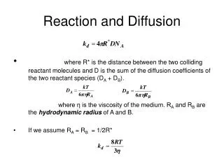
Reaction and Diffusion • where R* is the distance between the two colliding reactant molecules and D is the sum of the diffusion coefficients of the two reactant species (DA + DB). where η is the viscosity of the medium. RA and RB are the hydrodynamic radius of A and B. • If we assume RA = RB = 1/2R*
24.3 The material balance equation (a) The formulation of the equation the net rate of change due to chemical reactions the overall rate of change the above equation is called the material balance equation.
(b) Analytical solutions of the material balance equation Using numerical method: Euler method or 4th order Runge-Kutta method to Integrate the differential equation set.
Fig. 1 Snapshots of stationary 2D spots (A) and stripes (B) in a thin layer and 2D images of the corresponding 3D structures (A→B, C; B→E to G) in a capillary. T Bánsági et al. Science 2011;331:1309-1312 Published by AAAS
Fig. 3 Stationary structures in numerical simulations. Stationary structures in numerical simulations. Spots (A), hexagonal close-packing (B), labyrinthine (C), tube (D), half-pipe (E), and lamellar (F) emerging from asymmetric [(A), (B), and (E)], symmetric [(D) and (F)], and random (C) initial conditions in a cylindrical domain. Numerical results are obtained from the model: dx/dτ = (1/ε)[fz(q – x)/(q + x) + x(1 – mz)/(ε1 + 1 – mz) – x2] + ∇2x; dz/dτ = x(1 – mz)/(ε1 + 1 – mz) – z + dz∇2z, where x and z denote the activator, HBrO2 and the oxidized form of the catalyst, respectively; dz is the ratio of diffusion coefficients Dz/Dx; and τ is the dimensionless time. Parameters (dimensionless units): q = 0.0002; m = 0.0007; ε1 = 0.02; ε = 2.2; f = (A) 1.1, (B) 0.93, [(C) to (F)] 0.88; and dz = 10. Size of domains (dimensionless): diameter = 20 [(A) to (C) and (F)]; 14 [(D) and (E)]; height = 40. T Bánsági et al. Science 2011;331:1309-1312 Published by AAAS
Transition State Theory(Activated complex theory) • Using the concepts of statistical thermodynamics. • Steric factor appears automatically in the expression of rate constants.
24.4 The Eyring equation • The transition state theory pictures a reaction between A and B as proceeding through the formation of an activated complex in a pre-equilibrium: A + B ↔ C‡ ( `‡` is represented by `±` in the math style) • The partial pressure and the molar concentration have the following relationship: pJ = RT[J] • thus • The activated complex falls apart by unimolecular decay into products, P, C‡ → P v = k‡[C‡] • So Define v = k2[A][B]
(a) The rate of decay of the activated complex k‡ = κv where κ is the transmission coefficient. κ is assumed to be about 1 in the absence of information to the contrary. v is the frequency of the vibration-like motion along the reaction-coordinate.
(b) The concentration of the activated complex Based on Equation 17.54 (or 20.54 in 7th edition), we have with ∆E0 = E0(C‡) - E0(A) - E0(B) are the standard molar partition functions. provided hv/kT << 1, the above partition function can be simplified to Therefore we can write qC‡ ≈ where denotes the partition function for all the other modes of the complex. K‡ =
(c) The rate constant combine all the parts together, one gets then we get (Eyring equation) To calculate the equilibrium constant in the Eyring equation, one needs to know the partition function of reactants and the activated complexes. Obtaining info about the activated complex is a challeging task.
(d) The collisions of structureless particles A + B → AB Because A and B are structureless atoms, the only contribution to their partition functions are the translational terms:
Kinetics Salt Effect Ionic reaction A + B ↔ C‡ C‡ → P d[P]/dt = k‡[C‡] the thermodynamic equilibrium constant Then d[P]/dt = k2[A][B] Assuming is the rate constant when the activity coefficients are 1 ( ) Debye-Huckle limiting law with A = 0.509 log(k2) = log( ) + 2AZAZBI1/2 (Analyze this equation)
Example: The rate constant for the base hydrolysis of [CoBr(NH3)5]2+ varies with ionic strength as tabulated below. What can be deduced about the charge of the activated complex in the rate-determining stage? I 0.0050 0.0100 0.0150 0.0200 0.0250 0.0300 k/ko 0.718 0.631 0.562 0.515 0.475 0.447 Solution: I1/2 0.071 0.100 0.122 0.141 0.158 0.173 Log(k/ko) -0.14 -0.20 -0.25 -0.29 -0.32 -0.35
24.6 Reactive Collisions • Properties of incoming molecules can be controlled: 1. Translational energy. 2. Vibration energy. 3. Different orientations. • The detection of product molecules: 1. Angular distribution of products. 2. Energy distribution in the product.
24.7 Potential energy surface • Can be constructed from experimental measurements or from Molecular Orbital calculations, semi-empirical methods,……
Potential energy is a function of the relative positions of all the atoms taking Part in the reaction.
Crossing crowded dance floors. S Bradforth Science 2011;331:1398-1399 Published by AAAS
24.8 Results from experiments and calculations (a) The direction of the attack and separation