Download
1 / 27
450 likes | 836 Views
1 . /2. /2. H 0 : = 0. Acceptance Region for H 0. Rejection Region. Rejection Region. Power and Sample Size. “Null Distribution”.

E N D
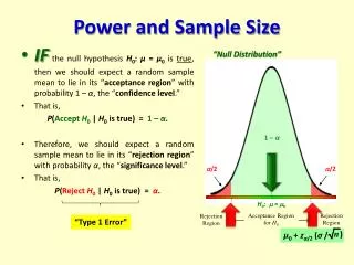
1 /2 /2 H0: = 0 Acceptance Region for H0 Rejection Region Rejection Region Power and Sample Size “Null Distribution” • IF the null hypothesis H0: μ = μ0is true, then we should expect a random sample mean to lie in its “acceptance region” with probability 1 – α, the “confidence level.” • That is, P(Accept H0 | H0 is true) = 1 – α. • Therefore, we should expect a random sample mean to lie in its “rejection region” with probability α, the “significance level.” • That is, P(Reject H0 | H0 is true) = α. “Type 1 Error” μ0+ zα/2(σ /
1 /2 /2 H0: = 0 Acceptance Region for H0 Rejection Region Rejection Region Power and Sample Size “Alternative Distribution” “Null Distribution” • IF the null hypothesis H0: μ = μ0is false, then the “power” to correctly reject it in favor of a particular alternative HA: μ = μ1is P(Reject H0 | H0 is false) = 1 – . Thus, P(AcceptH0 | H0 is false) = . 1 – HA: μ = μ1 Set them equal to each other, and solve for n… “Type 2 Error” μ1 –z(σ / μ0+ zα/2(σ /
Given: • X ~ N(μ, σ) Normally-distributed population random variable, with unknown mean, but known standard deviation • H0: μ = μ0Null Hypothesis value • HA: μ = μ1Alternative Hypothesis specific value • significance level (or equivalently, confidence level 1 –) • 1 – power (or equivalently, Type 2 error rate ) Then the minimum required sample size is: N(0, 1) 1 z z.025 = 1.96 Example:σ= 1.5 yrs, μ0= 25.4 yrs, = .05 Suppose it is suspected that currently, μ1= 26 yrs. Want more power! Want 90% powerof correctly rejecting H0 in favor of HA, if it is false = |26 – 25.4| / 1.5 = 0.4 z.10 = 1.28 1 – = .90 = .10 n 66 So… minimum sample size required is
Given: • X ~ N(μ, σ) Normally-distributed population random variable, with unknown mean, but known standard deviation • H0: μ = μ0Null Hypothesis value • HA: μ = μ1Alternative Hypothesis specific value • significance level (or equivalently, confidence level 1 –) • 1 – power (or equivalently, Type 2 error rate ) Then the minimum required sample size is: N(0, 1) 1 z z.025 = 1.96 Example:σ= 1.5 yrs, μ0= 25.4 yrs, = .05 Change μ1 Suppose it is suspected that currently, μ1= 26 yrs. Want 95% powerof correctly rejecting H0 in favor of HA, if it is false Want 90% powerof correctly rejecting H0 in favor of HA, if it is false = |26 – 25.4| / 1.5 = 0.4 z.10 = 1.28 1 – = .90 = .10 = .05 z.05 = 1.645 1 – = .95 n 82 n 66 So… minimum sample size required is
Given: • X ~ N(μ, σ) Normally-distributed population random variable, with unknown mean, but known standard deviation • H0: μ = μ0Null Hypothesis value • HA: μ = μ1Alternative Hypothesis specific value • significance level (or equivalently, confidence level 1 –) • 1 – power (or equivalently, Type 2 error rate ) Then the minimum required sample size is: N(0, 1) 1 z z.025 = 1.96 Example:σ= 1.5 yrs, μ0= 25.4 yrs, = .05 Suppose it is suspected that currently, μ1= 25.7 yrs. Suppose it is suspected that currently, μ1= 26 yrs. Want 95% powerof correctly rejecting H0 in favor of HA, if it is false = |25.7 – 25.4| / 1.5 = 0.2 = |31 – 30| / 2.4 = 0.41667 = .05 1 – = .95 z.05 = 1.645 n 325 n 82 So… minimum sample size required is
Given: • X ~ N(μ, σ) Normally-distributed population random variable, with unknown mean, but known standard deviation • H0: μ = μ0Null Hypothesis value • HA: μ = μ1Alternative Hypothesis specific value • significance level (or equivalently, confidence level 1 –) • 1 – power (or equivalently, Type 2 error rate ) Then the minimum required sample size is: N(0, 1) 1 z z.025 = 1.96 Example:σ= 1.5 yrs, μ0= 25.4 yrs, = .05 Suppose it is suspected that currently, μ1= 25.7 yrs. With n = 400, how much power exists to correctly reject H0 in favor of HA, if it is false? Power = 1 – = = 0.9793, i.e., 98%
Given: • X ~ N(μ, σ) Normally-distributed population random variable, with unknown mean, but known standard deviation • H0: μ = μ0Null Hypothesis • HA: μ ≠ μ0 Alternative Hypothesis (2-sided) • significance level (or equivalently, confidence level 1 –) • n sample size From this, we obtain… “standard error” s.e. sample mean sample standard deviation …with which to test the null hypothesis (via CI, AR, p-value). In practice however, it is far more common that the true population standard deviation σ is unknown. So we must estimate it from the sample! But this introduces additional variability from one sample to another… PROBLEM! (estimate) x1, x2,…, xn Recall that
Given: • X ~ N(μ, σ) Normally-distributed population random variable, with unknown mean, but known standard deviation • H0: μ = μ0Null Hypothesis • HA: μ ≠ μ0 Alternative Hypothesis (2-sided) • significance level (or equivalently, confidence level 1 –) • n sample size From this, we obtain… “standard error” s.e. sample mean sample standard deviation …with which to test the null hypothesis (via CI, AR, p-value). SOLUTION: follows a different sampling distribution from before. But this introduces additional variability from one sample to another… PROBLEM! (estimate) x1, x2,…, xn
Student’s T-Distribution … is actually a family of distributions, indexed by the degrees of freedom, labeled tdf. Z ~ N(0, 1) t10 t3 t2 William S. Gossett (1876 - 1937) t1 As the sample size n gets large, tdf converges to the standard normal distribution Z ~ N(0, 1). So the T-test is especially useful when n < 30.
Student’s T-Distribution … is actually a family of distributions, indexed by the degrees of freedom, labeled tdf. Z ~ N(0, 1) t4 William S. Gossett (1876 - 1937) .025 1.96 As the sample size n gets large, tdf converges to the standard normal distribution Z ~ N(0, 1). So the T-test is especially useful when n < 30.
Lecture Notes Appendix… or… qt(.025, 4, lower.tail = F) [1] 2.776445
Student’s T-Distribution … is actually a family of distributions, indexed by the degrees of freedom, labeled tdf. Z ~ N(0, 1) t4 William S. Gossett (1876 - 1937) .025 .025 1.96 2.776 Because any t-distribution has heavier tails than the Z-distribution, it follows that for the same right-tailed area value, t-score > z-score.
Given: X = Age at first birth~ N(μ, σ) • H0: μ = 25.4yrs Null Hypothesis • HA: μ ≠25.4 yrs Alternative Hypothesis Now suppose that σis unknown, and n < 30. Previously… σ= 1.5 yrs, n= 400, statistically significant at = .05 Example:n = 16, s = 1.22 yrs • standard error (estimate) = • .025 critical value = t15, .025
Given: X = Age at first birth~ N(μ, σ) • H0: μ = 25.4 yrs Null Hypothesis • HA: μ ≠25.4 yrs Alternative Hypothesis Now suppose that σis unknown, and n < 30. Previously… σ= 1.5 yrs, n= 400, statistically significant at = .05 Example:n = 16, s = 1.22 yrs 95% margin of error = (2.131)(0.305 yrs) = 0.65 yrs • standard error (estimate) = = 2.131 • .025 critical value = t15, .025 95% Confidence Interval = (25.9 – 0.65, 25.9 + 0.65) = (25.25, 26.55) yrs p-value = • Test Statistic:
Given: X = Age at first birth~ N(μ, σ) • H0: μ = 25.4 yrs Null Hypothesis • HA: μ ≠25.4 yrs Alternative Hypothesis Now suppose that σis unknown, and n < 30. Example:n = 16, s = 1.22 yrs Previously… σ= 1.5 yrs, n= 400, statistically significant at = .05 95% margin of error = (2.131)(0.305 yrs) = 0.65 yrs • standard error (estimate) = • .025 critical value = t15, .025 = 2.131 95% Confidence Interval = CONCLUSIONS: (25.9 – 0.65, 25.9 + 0.65) = The 95% CI does contain the null value μ = 25.4. (25.25, 26.55) yrs The p-value is between .10 and .20, i.e., > .05. (Note: The R command 2 * pt(1.639, 15, lower.tail = F) gives the exact p-value as .122.) p-value = = 2 (between .05 and .10) Not statistically significant; small n gives low power! = between .10 and .20.
Lecture Notes Appendix A3.3…(click for details on this section) AssumingX ~ N(, σ), test H0: = 0vs. HA: ≠0, at level α… AssumingX ~ N(, σ) To summarize… If the population variance 2 is known, then use it with the Z-distribution, for any n. • If the population variance 2 is unknown, then estimate it by the samplevariances 2, and use: • either T-distribution (more accurate), or the Z-distribution (easier), if n 30, • T-distribution only, if n < 30.
Lecture Notes Appendix A3.3…(click for details on this section) AssumingX ~ N(, σ), test H0: = 0vs. HA: ≠0, at level α… AssumingX ~ N(, σ) To summarize… If the population variance 2 is known, then use it with the Z-distribution, for any n. • If the population variance 2 is unknown, then estimate it by the samplevariances 2, and use: • either T-distribution (more accurate), or the Z-distribution (easier), if n 30, • T-distribution only, if n < 30.
How do we check that this assumption is reasonable, when all we have is a sample? And what do we do if it’s not, or we can’t tell? IF our data approximates a bell curve, then its quantiles should “line up” with those of N(0, 1). Z ~ N(0, 1) AssumingX ~ N(, σ)
How do we check that this assumption is reasonable, when all we have is a sample? And what do we do if it’s not, or we can’t tell? Sample quantiles IF our data approximates a bell curve, then its quantiles should “line up” with those of N(0, 1). Z ~ N(0, 1) • Q-Q plot • Normal scores plot • Normal probability plot AssumingX ~ N(, σ)
How do we check that this assumption is reasonable, when all we have is a sample? And what do we do if it’s not, or we can’t tell? IF our data approximates a bell curve, then its quantiles should “line up” with those of N(0, 1). • Q-Q plot • Normal scores plot • Normal probability plot AssumingX ~ N(, σ) qqnorm(mysample) (R uses a slight variation to generate quantiles…)
How do we check that this assumption is reasonable, when all we have is a sample? And what do we do if it’s not, or we can’t tell? IF our data approximates a bell curve, then its quantiles should “line up” with those of N(0, 1). • Q-Q plot • Normal scores plot • Normal probability plot AssumingX ~ N(, σ) qqnorm(mysample) (R uses a slight variation to generate quantiles…) Formal statistical tests exist; see notes.
How do we check that this assumption is reasonable, when all we have is a sample? And what do we do if it’s not, or we can’t tell? • Use a mathematical “transformation” of the data (e.g., log, square root,…). x = rchisq(1000, 15) hist(x) y = log(x) hist(y) X is said to be “log-normal.” AssumingX ~ N(, σ)
How do we check that this assumption is reasonable, when all we have is a sample? And what do we do if it’s not, or we can’t tell? • Use a mathematical “transformation” of the data (e.g., log, square root,…). qqnorm(x, pch = 19, cex = .5) qqnorm(y, pch = 19, cex = .5) AssumingX ~ N(, σ)
How do we check that this assumption is reasonable, when all we have is a sample? And what do we do if it’s not, or we can’t tell? • Use a mathematical “transformation” of the data (e.g., log, square root,…). • Use a “nonparametric test” (e.g., Sign Test, Wilcoxon Signed Rank Test). = Mann-Whitney Test • Makes no assumptions on the underlying population distribution! • Based on “ranks” of the ordered data; tedious by hand… • Has less power than Z-test or T-test (when appropriate)… but not bad. AssumingX ~ N(, σ) • In R, see ?wilcox.testfor details…. SEE LECTURE NOTES, PAGE 6.1-27 FOR SUMMARY OF METHODS