Power and Sample Size
Power and Sample Size. Boulder 2004 Benjamin Neale Shaun Purcell. I HAVE THE POWER!!!. To be accomplished. Introduce power via e xample Identify factors relevant to power Practical: Empirical power analysis of ACE twin model How to use Mx for power. Simple example.


Power and Sample Size
E N D
Presentation Transcript
Power and Sample Size Boulder 2004 Benjamin Neale Shaun Purcell I HAVE THE POWER!!!
To be accomplished • Introduce power via example • Identify factors relevant to power • Practical: • Empirical power analysis of ACE twin model • How to use Mx for power
Simple example • Investigate the linear relationship (r) • between two random variables X and Y: • We are testingr=0 vs.r0
How to investigate r • Draw a sample, measure X,Y • Calculate the measure of association r (Pearson product moment corr. coeff.) • Test whether r 0.
How to Test r 0 • Assumed data are normally distributed • Define a null-hypothesis (r = 0) • Chose a level (usually .05) • Assume (null) distribution of the test statistic (t) associated with r=0 • t=r [(N-2)/(1-r2)]
How to Test r 0 • Sample N=40 • r=.303, t=1.867, df=38, p=.06 α=.05 • As p > α, we fail to reject r= 0 • Have we drawn the correct conclusion?
A note on a • Type I error rate = a • probability of deciding r 0 (while in truth r=0) • Usually a is .05...why? DOGMA
N=40, r=0, nrep=1000 – central t(38), a=0.05 (critical value 2.04)
In 23% of tests of r=0, |t|>2.024 (a=0.05), and thus draw the correct conclusion that of rejecting r =0. The probability of rejecting the null-hypothesis (r=0) correctly is 1-b, or the power, when a true effect exists
Hypothesis Testing • Correlation Coefficient hypotheses: • ho (null hypothesis) is ρ=0 • ha (alternative hypothesis) is ρ≠ 0 • Two-sided test, where ρ > 0 or ρ < 0 are one-sided • Null hypothesis usually assumes no effect • Alternative hypothesis is the idea being tested
Summary of Possible Results H-0 true H-0 false accept H-0 1-ab reject H-0 a 1-b a=type 1 error rate b=type 2 error rate 1-b=statistical power
Type I error at rate Nonsignificant result (1- ) Type II error at rate Significant result (1-) STATISTICS Non-rejection of H0 Rejection of H0 H0 true R E A L I T Y HA true
Power • The probability of rejection of a false null-hypothesis depends on: • the significance criterion () • the sample size (N) • the effect size (NCP) “The probability of detecting a given effect size in a population from a sample of size N, using significance criterion ”
Standard Case Sampling distribution if HA were true Sampling distribution if H0 were true P(T) alpha 0.05 POWER = 1 - T Effect Size (NCP)
Impact of Less Cons. alpha Sampling distribution if HA were true Sampling distribution if H0 were true P(T) alpha 0.1 POWER = 1 - T
Impact of More Cons. alpha Sampling distribution if HA were true Sampling distribution if H0 were true P(T) alpha 0.01 POWER = 1 - T
Increase in Sample Size Sampling distribution if HA were true Sampling distribution if H0 were true P(T) alpha 0.05 POWER = 1 - T Effect Size (NCP)↑
Increase in Effect Size Sampling distribution if HA were true Sampling distribution if H0 were true P(T) alpha 0.05 POWER = 1 - T Effect Size (NCP)↑
Effects on Power Recap • Larger Effect Size • Larger Sample Size • Alpha Level shifts <Beware the False Positive!!!> • Type of Data: • Binary, Ordinal, Continuous
When To Do Power Calcs? • Generally study planning stages of study • Occasionally with negative result • No need if significance is achieved • Computed to determine chances of success
Power Calculations Empirical • Attempt to Grasp the NCP from Null • Simulate Data under theorized model • Calculate Statistics and Perform Test • Given α, how many tests p < α • Power = (#hits)/(#tests)
Practical: Empirical Power 1 • We will Simulate Data under a model online • We will run an ACE model, and test for C • We will then submit our data and Shaun will collate it for us • While he’s collating, we’ll talk about theoretical power calculations
Practical: Empirical Power 2 • First get F:\ben\2004\ace.mx and put it into your directory • We will paste our simulated data into this script, so open it now in preparation, and note both places where we must paste in the data • Note that you will have to fit the ACE model and then fit the AE submodel
Practical: Empirical Power 3 • Simulation Conditions • 30% A2 20% C2 50% E2 • Input: • A 0.5477 C of 0.4472 E of 0.7071 • 350 MZ 350 DZ • Simulate and Space Delimited at • http://statgen.iop.kcl.ac.uk/workshop/unisim.html or click here in slide show mode • Click submit after filling in the fields and you will get a page of data
Practical: Empirical Power 4 • With the data page, use control-a to select the data, control-c to copy, and in Mx control-v to paste in both the MZ and DZ groups. • Run the ace.mx script with the data pasted in and modify it to run the AE model. • Report the A, C, and E estimates of the first model, and the A and E estimates of the second model as well as both the -2log-likelihoods on the webpage http://statgen.iop.kcl.ac.uk/workshop/ or click here in slide show mode
Practical: Empirical Power 5 • Once all of you have submitted your results we will take a look at the theoretical power calculation, using Mx. • Once we have finished with the theory Shaun will show us the empirical distribution that we generated today
Theoretical Power Calculations • Based on Stats, rather than Simulations • Can be calculated by hand sometimes, but Mx does it for us • Note that sample size and alpha-level are the only things we can change, but can assume different effect sizes • Mx gives us the relative power levels at the alpha specified for different sample sizes
Theoretical Power Calculations • We will use the power.mx script to look at the sample size necessary for different power levels • In Mx, power calculations can be computed in 2 ways: • Using Covariance Matrices (We Do This One) • Requiring an initial dataset to generate a likelihood so that we can use a chi-square test
Power.mx 1 ! Simulate the data ! 30% additive genetic ! 20% common environment ! 50% nonshared environment #NGroups 3 G1: model parameters Calculation Begin Matrices; X lower 1 1 fixed Y lower 1 1 fixed Z lower 1 1 fixed End Matrices; Matrix X 0.5477 Matrix Y 0.4472 Matrix Z 0.7071 Begin Algebra; A = X*X' ; C = Y*Y' ; E = Z*Z' ; End Algebra; End
Power.mx 2 G2: MZ twin pairs Calculation Matrices = Group 1 Covariances A+C+E | A+C _ A+C | A+C+E / Options MX%E=mzsim.cov End G3: DZ twin pairs Calculation Matrices = Group 1 H Full 1 1 Covariances A+C+E | H@A+C _ H@A+C | A+C+E / Matrix H 0.5 Options MX%E=dzsim.cov End
Power.mx 3 ! Second part of script ! Fit the wrong model to the simulated data ! to calculate power #NGroups 3 G1 : model parameters Calculation Begin Matrices; X lower 1 1 free Y lower 1 1 fixed Z lower 1 1 free End Matrices; Begin Algebra; A = X*X' ; C = Y*Y' ; E = Z*Z' ; End Algebra; End
Power.mx 4 G2 : MZ twins Data NInput_vars=2 NObservations=350 CMatrix Full File=mzsim.cov Matrices= Group 1 Covariances A+C+E | A+C _ A+C | A+C+E / Option RSiduals End G3 : DZ twins Data NInput_vars=2 NObservations=350 CMatrix Full File=dzsim.cov Matrices= Group 1 H Full 1 1 Covariances A+C+E | H@A+C _ H@A+C | A+C+E / Matix H 0.5 Option RSiduals ! Power for alpha = 0.05 and 1 df Option Power= 0.05,1 End