Power and Sample Size

1. Power and Sample Size Adapted from: Boulder 2004 Benjamin Neale Shaun Purcell I HAVE THE POWER!!!

2. Overview • Introduce Concept of Power via Correlation Coefficient (ρ) Example • Discuss Factors Contributing to Power • Practical: • Simulating data as a means of computing power • Using Mx for Power Calculations

3. Simple example • Investigate the linear relationship between two random variables X and Y: ρ=0 vs. ρ≠0 • using the Pearson correlation coefficient. • Sample subjects at random from population • Measure X andY • Calculate the measure of association ρ • Test whether ρ≠ 0. 3

4. How to Test ρ≠ 0 • Assume data are normally distributed • Define a null-hypothesis (ρ = 0) • Choose an α level (usually .05) • Use the (null) distribution of the test statistic associated with ρ=0 • t=ρ√ [(N-2)/(1-ρ2)] 4

5. How to Test ρ≠ 0 • Sample N=40 • r=.303, t=1.867, df=38, p=.06 α =.05 • Because observed p > α, we fail to reject ρ = 0 • Have we drawn the correct conclusion that p is genuinely zero? 5

6. DOGMA = type I error rate probability of deciding ρ ≠ 0(while in truth ρ=0)α is often chosen to equal .05...why? 6

7. N=40, r=0, nrep=1000, central t(38), α=0.05 (critical value 2.04) 7

8. Observed non-null distribution (ρ=.2) and null distribution 8

9. In 23% of tests that ρ=0, |t|>2.024 (α=0.05), and thus correctly conclude that ρ = 0. The probability of correctly rejecting the null-hypothesis (ρ=0) is 1-β, known as the power. 9

10. Hypothesis Testing • Correlation Coefficient hypotheses: • ho (null hypothesis) is ρ=0 • ha (alternative hypothesis) is ρ ≠ 0 • Two-sided test, where ρ > 0 or ρ < 0 are one-sided • Null hypothesis usually assumes no effect • Alternative hypothesis is the idea being tested

11. Summary of Possible Results • H-0 true H-0 false • accept H-0 1-αβ • reject H-0 α1-β • α=type 1 error rate • β=type 2 error rate • 1-β=statistical power 11

12. Nonsignificant result (1- α) Type II error at rate β Significant result (1-β) Type I error at rate α STATISTICS Non-rejection of H0 Rejection of H0 H0 true R E A L I T Y HA true

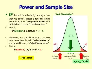
13. Power • The probability of rejecting the null-hypothesis depends on: • the significance criterion (α) • the sample size (N) • the effect size (NCP) “The probability of detecting a given effect size in a population from a sample of size N, using significance criterion α”

14. Standard Case Sampling distribution if HA were true Sampling distribution if H0 were true P(T) alpha 0.05 POWER = 1 - β α β T Effect Size (NCP)

15. Impact of less conservative α Sampling distribution if HA were true Sampling distribution if H0 were true P(T) alpha 0.1 POWER = 1 - β↑ α T β

16. Impact of more conservative α Sampling distribution if HA were true Sampling distribution if H0 were true P(T) alpha 0.01 POWER = 1 - β↓ α T β

17. Impact of increased sample size Reduced variance of sampling distribution if HA is true Sampling distribution if H0 is true P(T) alpha 0.05 POWER = 1 - β↑ α T β

18. Impact of increase in Effect Size Sampling distribution if HA were true Sampling distribution if H0 were true P(T) alpha 0.05 POWER = 1 - β↑ α β T Effect Size (NCP)↑

19. Summary: Factors affecting power • Effect Size • Sample Size • Alpha Level • <Beware the False Positive!!!> • Type of Data: • Binary, Ordinal, Continuous • Research Design

20. Uses of power calculations • Planning a study • Possibly to reflect on ns trend result • No need if significance is achieved • To determine chances of study success

21. Power Calculations via Simulation • Simulate Data under theorized model • Calculate Statistics and Perform Test • Given α, how many tests p < α • Power = (#hits)/(#tests)

22. Practical: Empirical Power 1 • Simulate Data under a model online • Fit an ACE model, and test for C • Collate fit statistics on board

23. Practical: Empirical Power 2 • First get http://www.vipbg.vcu.edu/neale/gen619/power/power-raw.mx and put it into your directory • Second, open this script in Mx, and note both places where we must paste in the data • Third, simulate data (see next slide) • Fourth, fit the ACE model and then fit the AE submodel

24. Practical: Empirical Power 3 • Simulation Conditions • 30% A2 20% C2 50% E2 • Input: • A 0.5477 C of 0.4472 E of 0.7071 • 350 MZ 350 DZ • Simulate and use “Space Delimited” option at • http://statgen.iop.kcl.ac.uk/workshop/unisim.html or click here in slide show mode • Click submit after filling in the fields and you will get a page of data

25. Practical: Empirical Power 4 • With the data page, use ctrl-a to select the data, control-c to copy, switch to Mx (e.g. with alt-tab) and in Mx control-v to paste in both the MZ and DZ groups. • Run the ace.mx script with the data pasted in and modify it to run the AE model. • Report the -2log-likelihoods on the whiteboard • Optionally, keep a record of A, C, and E estimates of the first model, and the A and E estimates of the second model

26. Simulation of other types of data • Use SAS/R/Matlab/Mathematica • Any decent random number generator will do • See http://www.vipbg.vcu.edu/~neale/gen619/power/sim1.sas

27. R • R is in your future • Can do it manually with rnorm • Easier to use mvrnorm • runmx at Matt Keller’s site: • http://www.matthewckeller.com/html/mx-r.html library (MASS) mvrnorm(n=100,c(1,1),matrix(c(1,.5,.5,1),2,2),empirical=FALSE) 27

28. Mathematica Example In[32]:= (mu={1,2,3,4}; sigma={{1,1/2,1/3,1/4},{1/2,1/3,1/4,1/5},{1/3,1/4,1/5,1/6},{1/4,1/5,1/6, 1/7}}; Timing[Table[Random[MultinormalDistribution[mu,sigma]],{1000}]][[1]]) Out[32]= 1.1 Second In[33]:= Timing[RandomArray[MultinormalDistribution[mu,sigma],1000]][[1]] Out[33]= 0.04 Second In[37]:= TableForm[RandomArray[MultinormalDistribution[mu,sigma],10]] Obtain mathematica from VCU http://www.ts.vcu.edu/faq/stats/mathematica.html

29. Theoretical Power Calculations • Based on Stats, rather than Simulations • Can be calculated by hand sometimes, but Mx does it for us • Note that sample size and alpha-level are the only things we can change, but can assume different effect sizes • Mx gives us the relative power levels at the alpha specified for different sample sizes

30. Theoretical Power Calculations • We will use the power.mx script to look at the sample size necessary for different power levels • In Mx, power calculations can be computed in 2 ways: • Using Covariance Matrices (We Do This One) • Requiring an initial dataset to generate a likelihood so that we can use a chi-square test

31. Power.mx 1 ! Simulate the data ! 30% additive genetic ! 20% common environment ! 50% nonshared environment #NGroups 3 G1: model parameters Calculation Begin Matrices; X lower 1 1 fixed Y lower 1 1 fixed Z lower 1 1 fixed End Matrices; Matrix X 0.5477 Matrix Y 0.4472 Matrix Z 0.7071 Begin Algebra; A = X*X' ; C = Y*Y' ; E = Z*Z' ; End Algebra; End

32. Power.mx 2 G2: MZ twin pairs Calculation Matrices = Group 1 Covariances A+C+E | A+C _ A+C | A+C+E / Options MX%E=mzsim.cov End G3: DZ twin pairs Calculation Matrices = Group 1 H Full 1 1 Covariances A+C+E | H@A+C _ H@A+C | A+C+E / Matrix H 0.5 Options MX%E=dzsim.cov End

33. Power.mx 3 ! Second part of script ! Fit the wrong model to the simulated data ! to calculate power #NGroups 3 G1 : model parameters Calculation Begin Matrices; X lower 1 1 free Y lower 1 1 fixed Z lower 1 1 free End Matrices; Begin Algebra; A = X*X' ; C = Y*Y' ; E = Z*Z' ; End Algebra; End

34. Power.mx 4 G2 : MZ twins Data NInput_vars=2 NObservations=350 CMatrix Full File=mzsim.cov Matrices= Group 1 Covariances A+C+E | A+C _ A+C | A+C+E / Option RSiduals End G3 : DZ twins Data NInput_vars=2 NObservations=350 CMatrix Full File=dzsim.cov Matrices= Group 1 H Full 1 1 Covariances A+C+E | H@A+C _ H@A+C | A+C+E / Matix H 0.5 Option RSiduals ! Power for alpha = 0.05 and 1 df Option Power= 0.05,1 End

35. Model Identification • Necessary Conditions • Sufficient Conditions • Algebraic Tests • Empirical Tests 35

36. Necessary Conditions • Number of Parameters < or = Number of Statistics • Structural Equation Model usually count variances & covariances to identify variance components • What is the number of statistics/parameters in a univariate ACE model? Bivariate? 36

37. Sufficient Conditions • No general sufficient conditions for SEM • Special case: ACE model • Distinct Statistics (i.e. have different predicted values • VP = a2 + c2 + e2 • CMZ = a2 + c2 • CDZ = .5 a2 + c2 37

38. Sufficient Conditions 2 • Arrange in matrix form • 1 1 1 a2 VP • 1 1 0 c2 = CMZ • .5 1 0 e2 CDZ • A x = b • If A can be inverted then can find A-1b 38

39. Sufficient Conditions 3 Solve ACE modelCalc ng=1Begin Matrices; A full 3 3 b full 3 1End Matrices;Matrix A1 1 11 1 0.5 1 0Labels Col A A C ELabels Row A VP CMZ CDZ Matrix b ! Data, essentially1.8.5Labels Col B StatisticLabels Row B VP CMZ CDZBegin Algebra; C = A~; x = A~*b;End Algebra;Labels Row x A C EEnd 39

40. Sufficient Conditions 4 • What if not soluble by inversion? • Empirical: • 1 Pick set of parameter values T1 • 2 Simulate data • 3 Fit model to data starting at T2 (not T1) • 4 Repeat and look for solutions to step 3 that are perfect but have estimates not equal to T1 • If equally good solution but different values, reject identified model hypothesis 40

41. Conclusion • Power calculations relatively simple to do • Curse of dimensionality • Different for raw vs summary statistics • Simulation can be done many ways • No substitute for research design