Immersed Boundary Method
Immersed Boundary Method. Presentation for Lab meeting February 15, 2006 Michalis Xenos and Andreas Linninger Laboratory for Product and Process Design , Department of Chemical Engineering, University of Illinois, Chicago, IL 60607, U.S.A.


Immersed Boundary Method
E N D
Presentation Transcript
Immersed Boundary Method Presentation for Lab meeting February 15, 2006 Michalis Xenos and Andreas Linninger Laboratory for Product and Process Design, Department of Chemical Engineering, University of Illinois, Chicago, IL 60607, U.S.A.
Immersed Boundary Method(IBM) – IntroductionR. Mittal, G. Iaccarino The term “immersed boundary method” was first used in reference to a method developed by Peskin (1972) to simulate cardiac mechanics and associated blood flow. The distinguishing feature of this method was that the entire simulation was carried out on a Cartesian grid, which did not conform to the geometry of the heart, and a novel procedure was formulated for imposing the effect of the immersed boundary (IB) on the flow. Since Peskin introduced this method, numerous modifications and refinements have been proposed and a number of variants of this approach now exist. Application of these and related methods to problems with liquid-liquid and liquid-gas boundaries (Volume of Fluid method – Front Tracking method).
Imposition of boundary conditions on IBM Figure 1 (a) Schematic showing a generic body past which flow is to be simulated. The body occupies the volume Ωbwith boundary Γb. The body has a characteristic length scale L, and a boundary layer of thickness δ develops over the body. (b) Schematic of body immersed in a Cartesian grid on which the governing equations are discretized.
Imposition of boundary conditions on IB • For ease of discussion, the coupled system of momentum and continuity equations can be notionally written as where U = (u, p) and L is the operator representing the Navier-Stokes equations as in Equation 1. • It should be noted that in the context of the incompressibleNavier-Stokes equations, pressure is determined by the continuity constraint and,consequently, the continuity equation is considered an implicit equation for pressure. • A number of numerical integration schemes such as fractional-step (Chorin1968) and SIMPLE (Patankar 1980) also explicitly derive and solve a Poissonequation for pressure, which, depending on the particular implementation, alsorequires appropriate boundary conditions.
Imposition of boundary conditions on IB • Continuous forcing approach • In the first implementation, the forcing function, denoted here by fb, is included into the continuous governing Eq. (3) leading to the equation L(U) = f b, which then applies to the entire domain (Ωf+Ωb). Note that f b= ( fm, fp) where fmand fpare the forcing functions applied to the momentum and pressure, respectively. This equation is subsequently discretized on a Cartesian grid, leading to the following system of discrete equations: • and this system of equations is solved in the entire domain • Discrete forcing approach • In this second approach, the governing equations are first discretized on a Cartesian grid without regard to the immersed boundary, resulting in the set of discretized equations [L] {U} = 0. Following this, the discretization in the cells near the IB is adjusted to account for its presence, resulting in a modified system of equations [L’ ]{U} = {r }, which are then solved on the Cartesian grid.
Continuous Forcing Approach • Flows with Elastic Boundaries In this method the fluid flow is governed by the incompressible Navier-Stokes equations and these are solved on a stationary Cartesian grid. The IB is represented by a set of elastic fibers and the location of these fibers is tracked in a Lagrangian fashion by a collection of mass-less points that move with the local fluid velocity. Thus, the coordinate Xkof the kth Lagrangian point is governed by the equation The stress (denoted by F) and deformation of these elastic fibers is related by a constitutive law such as the Hooke’s law. The effect of the IB on the surrounding fluid is essentially captured by transmitting the fiber stress to the fluid through a localized forcing term in the momentum equations, which is given by where δ is the Dirac delta function. Figure 2 (a) Transfer of forcing Fkfrom Lagrangian boundary point ( Xk) to surrounding fluid nodes. Shaded region signifies the extent of the force distribution. (b) Distribution functions employed in various studies.
Continuous Forcing Approach • Flows with Rigid Boundaries This problem could be circumvented by considering the body to be elastic but extremely stiff. A second approach is to consider the structure attached to an equilibrium location (Beyer & Leveque 1992, Lai & Peskin 2000) by a spring with a restoring force F given by where κ is a positive spring constant and Xekis the equilibrium location of the kth Lagrangian point. Accurately imposing the boundary condition on the rigid IB requires large values of κ.
Discrete Forcing Approach • Direct BC Imposition CHOST CELL FINITE-DIFFERENCE APROACH & CUT-CELL FINITE-VOLUME APPROACH. For each ghost cell, an interpolation scheme that implicitly incorporates the boundary condition on the IB is then devised. A number of options are available for constructing the interpolation scheme (Majumdar et al. 2001). One simple option is bilinear (trilinear in 3D) interpolation where a generic flow variable φ can be expressed with reference to Figure 3 as The four coefficients in the above equation can be evaluated in terms of the values of φ at fluid nodes F1, F2, and F3, and at the boundary point B2, which is the normal intercept from the ghost node to the IB. Figure 3 Representation of the points in the vicinity of an immersed boundary used in the ghost-cell approach. Fi are fluid points, G is the ghost point, and Bi and Pi are locations where the boundary condition can be enforced.
Flows with moving boundaries Figure 4 Schematics showing the key features of the cut-cell methodology. (a) Trapezoidal finite volume formed near the immersed boundary for which f denotes the face-flux of a generic variable. (b) Region of interpolation and stencil employed for approximating the flux fsw on the southwest face of the trapezoidal finite volume. Figure 5 Schematic showing the creation of “freshly-cleared” cells on a fixed Cartesian grid due to boundary motion from time step (t −t) to t. Schematic indicates how the flow variables at one such cell could be obtained by interpolating from neighboring nodes and from the immersed boundary.
Applications • Flow past flapping filaments • Flow past a pick-up truck • Flow past a sphere • Flutter and tumble of bodies in free fall This simulation employed a uniform 900×1200 Cartesian grid and took approximately 50 CPU hours on a single processor 733 MHz Alpha workstation.