Download
1 / 43
430 likes | 542 Views
Ocean-Coast Exchange Processes and SeaSonde Mapping Mike Kosro, COAS/Oregon State University. What processes carry water across shore? What are their time and space scales? How do we detect them? Gyre-scale circulation: West Wind Drift and its split

E N D
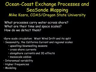
Ocean-Coast Exchange Processes and SeaSonde MappingMike Kosro, COAS/Oregon State University • What processes carry water across shore? What are their time and space scales? How do we detect them? • Gyre-scale circulation: West Wind Drift and its split • Seasonality, the California Current and regional scales • upwelling/downwelling seasons • cross-shore currents • alongshore currents and 3D effects • mesoscale eddies • Interannual variability • Higher frequencies • Modeling
50°N 40°N 30°N Gyre-Scale Circulation On the largest scales, the basin-scale ocean gyres transport surface water toward shore in the West Wind Drift. Kirwan, et al, 1978 • “ West Wind Drift” carries surface waters toward the west coast, where it splits to north or south. • Latitude of split varies seasonally and interannually.
Wind-Driven Circulation • Winds are a primary forcing mechanism for ocean circulation. (Buoyancy forcing and tides are others). • Wind-driven surface transport is to the right of the (steady) winds. • Along the west coast, equatorward winds produce coastal upwelling through offshore surface flow. Poleward winds produce coastal downwelling through onshore surface flow. On average, these Ekman currents are weak, but can be strong in storms.
Wind-Driven Circulation, cont • Because cross-shore flows rearrange the density field, geostrophic flows arise. Equatorward (upwelling) winds produce an equatorward current jet, and poleward winds result in poleward currents. • These alongshore currents can develop instabilities, meander, form eddies, turning strong alongshore flows into strong cross-shore ones. • The alongshore flows also respond to bottom topography, and can be turned on/off shore.
Satellite Measured Winds: Jan Avg Risien & Chelton
Satellite Measured Winds: July Avg. Risien & Chelton
Time-Series Measurements Long-term observations of circulation and water properties off Oregon. Long-term Mooring (NH10): 1997-present Newport Hydro Line: 1961-1971 & 1997-present Surface Current Mapping: 1997-present
Summer/Winter average cross-section on Newport Line (T, S) Summer: Upwelling.offshore flow at surface, onshore flow deeper. Note surfacing at coast of properties from down to 200m. Produces an alongshore current jet. Winter: Downwelling.onshore flow, pushing surface waters down near the coast. Also note vertical mixing. Produces a poleward alongshore current. Smith, Kosro, Huyer, Fleischbein, 2006.
4 GLOBEC Mooring Sites: • Newport(44.65 N, 81m depth) • Coos Bay (43.16 N, 97m) • Rogue River (42.44 N, 76m) • Gray’s Harbor (46.86 N, 25m) Long-Term Midshelf Time-Series MeasurementsKosro, Hickey, Ramp, Letelier • Each mooring continuously recorded measurements of: • ADCP current profiles • T and S at fixed depths • chlorophyll fluorescence near 20m Duration: 4.5 to 7 yrsSampling Δt: 60 mins – 3 mins
Fall Winter Spring Summer Midshelf Temperature T : 4.5 yrs, 11 depths *Spring upwelling: onshore flow at depth, seen as cold water builds from depth. *Fall downwelling: onshore flow initially at surface, as warm water builds from surface.
Fall Winter Spring Summer MidshelfAlongshore Flow v(z) : 7 yrs ADCP profiles Fall/winter: Alongshore flow mostly poleward (red/yellow). Spring/summer: Alongshore flow mostly equatorward (blue/green)
Seasonal Cycle: Alongshore Current at Midshelf v(z) : 7 yrs ADCP profiles Winter Spring Summer Fall Poleward Equatorward Jet Poleward Equatorward Jet (implied upwelling, offshore at surface, onshore below) in spring/summer Poleward Flow (implied downwelling, onshore flow at surface, offshore below) in fall/winter.
Fall Winter Spring Summer u(z) : 7 yrs ADCP profiles MidshelfCross-shore Flow Unlike alongshore flow, it is difficult to see the on/offshore flow seasonality in the day-to-day time series.
Seasonal Cycle: Cross-shore current at Midshelf u(z) : 7 yrs ADCP profiles Winter Spring Summer Fall Cross-shore average is an order of magnitude weaker than alongshore avg. Upwelling (offshore surface flow) in spring/summer. Onshore flow is at mid-water. Downwelling (onshore surface flow, offshore deep flow) in fall/winter.
What about variation alongshore? • How do conditions vary from location to location alongshore? • in the ocean “weather” (day-to-day)? • in the ocean statistics (on average)? • Use mapping tool to examine this.
Long Range Array • 180 km range , 5 MHz maps every 1-3 hrs6 km ΔR, 5 deg. azimuth • Cape Blanco region, 2 sites, 2001 • Winchester Bay, added 8/2001 • Yaquina Head, added 8/2002 • Manhattan Beach added 5/2004 Loomis Lake added 5/2004
Standard Range Array • 40 km range, 12MHzhourly maps2 km ΔR, 5 deg. azimuth • 2 high-resolution regions: • Columbia River mouth – 2 sites • Newport/Heceta Bank – 3 sites • In Kosro(2005), showed that • core of the average coastal jet centered farther from shore as shelf widens from north to south • as the jet core moves offshore, a new jet repeatedly spins up inshore.
Avg. Seasonal Cycle, 2001-2005 • 1st examine full-record monthly averages • Watch spin-up of coastal jet • Watch development of cross-shore flow as season progresses. • Then, interannual variability, comparing monthly averages between years.
Apr May Spring Av ST = 4/4 Mar
July Aug Summer June
Oct Nov Fall Sep
Jan Feb Winter Dec
Interannual Variability: Apr 2001 2002 2003 2004 2005 2002, stronger than usual upwelling [“subarctic invasion”] 2003, 2005: delayed upwelling
Interannual Variability: May 2001 2002 2003 2004 2005 2002, stronger than usual upwelling [“subarctic invasion”] 2005: upwelling still delayed
Interannual Variability: June 2001 2002 2003 2004 2005 2005: alongshore jet now seen, but “late”: inshore of its usual cross-shelf location. Delayed start to upwelling brought low productivity at coast, bird die-offs, warm anomalies between Canada and Pt. Conception.
Eddies and Meanders:Mesoscale Variability Eddies can interact with the coastal flow, producing strong, very local, cross-shore flows.
Eddies over the slope and deep sea Eddies are large vortex features; typically have diameters of 30 km or more. These are the ocean analogue of storms in the atmosphere. When they lie near the continental shelf, they can interact with the shelf flow, enhancing exchange between the shelf and the deep ocean. Eddies can form transient closed eco-systems.
Eddies affect biological distributions Cover image, “Biological Oceanography”, C. Miller Off British Columbia coast Satellite image (Coastal Zone Color Scanner) enhanced to estimate chlorophyll concentrations. Eddy effects are prominent off the west coast: entraining, perhaps enhancing.
Eddies can form transient ecosystems Measurements near Santa Barbara, CA, by Washburn andNishimoto. Red = number of fish caught per net haul.A large spike appears near the center of the eddy(note current arrows).
A A B B C C A? B C 12/27/02 01/16 12/17/02 01/06/03 Eddies, Winter 2003 Satellite altimeter measures sea surface height. Red regions are high sea level, corresponding to CW eddies, A,B,&C. North side of eddies -> onshore flow. Note persistence of onshore flow from Eddy C, between Cape Blanco and Crescent City. A A B B C C 01/26 02/05 02/15 02/25 A B C Strub
Winter 2003: long-lived, localized onshore flow Jan 5 Jan 16 Jan 27 Jan 31 Kosro
Observational Summary • West-wind drift => shoreward transport • Ekman transport => slow on/offshore transport at the surface (also at bottom) depending on the wind (current) • Alongshore currents are much stronger, and can be turned cross-shore by topography or by meanders/instability. Strong seasonal component to this process at monthly time scales. • Eddies can produce strong cross-shore transport, and can be long-lived. They can be found outside of known “retention zones”.
Model Assimilation of HF Measurements • Models provide circulation estimates at high resolution in horizontal, vertical and time, beyond that possible from observations alone. • Data assimilation: uses measurements (e.g. HF-measured currents) to keep model simulation “on track”. • OSU group has developed statistical model for estimating subsurface currents and water properties based on surface currents.
Measurements help detailed numerical models of the coastal circulation – keeping the models “on track”. The model, in turn, extends the surface measurements into the ocean subsurface.
Assimilation of surface data improves model comparison w/ independent data at depth: Correlation Phase Models are still imperfect at reproducing observations exactly, but models informed by data assimilation are closer to observations, even away from the observations. • with assimilation of surface data • without data assimilation
Long Range Array • 180 km range , 5 MHz maps every 1-3 hrs6 km ΔR, 5 deg. azimuth • Cape Blanco region, 2 sites, 2001 • Winchester Bay, added 8/2001 • Yaquina Head, added 8/2002 • Manhattan Beach added 5/2004 Loomis Lake added 5/2004 • To North:Proposed extension north to the Canadian border is anticipated under NSF-ORION
Alongshore Current Jet and Topography Over the shelf, there is a strong tendency for the currents, even at the surface, to follow the bottom contours. Here, the alongshore jet is being steered away from shore by the widening of the continental shelf south of 44.8° N.