Download
1 / 54
960 likes | 2.75k Views
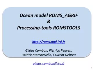
Ocean model ROMS_AGRIF & Processing-tools ROMSTOOLS http://roms.mpl.ird.fr Gildas Cambon , Pierrick Penven , Patrick Marchesiello , Laurent Debreu gildas.cambon@ird.fr. Ocean modeling principle. If we know: The ocean state at time t ( u,v,w,T,S , …)

E N D
Ocean model ROMS_AGRIF & Processing-tools ROMSTOOLS http://roms.mpl.ird.fr GildasCambon, PierrickPenven, Patrick Marchesiello, Laurent Debreu gildas.cambon@ird.fr
Ocean modeling principle • If we know: • The ocean state at time t (u,v,w,T,S, …) • Boundary conditions (surface, bottom, lateralsides) • Wecancompute the ocean state at t+dtusingnumerical approximations of Primitive Equations • For that we need to proceed discretization of the equations in time and space: Example of a finite difference grid
Introduction • Why use of ocean model : • Cost effective • Synoptic view • Equilibrium diagnostics • Test hypothesis • Hindcast and forecast • Coupling with different models • … Downloaded from Miami Isopycnic Coordinate model website 4-AGRIF nested grid, SST. Marchesiello et al, Ocean modelling, 2011.
Introduction • Equations to solve: • Navier Stoke equations but with approximations ! • Hypothesis: • Hydrostatic : H/L <<1, (aspect ratio low) • neglect vertical acceleration • neglectCoriolis termassociated to vertical velocities • Water is incompressible • Boussinesq : ρ=ρo=cste for horizontal gradient pressure Primitive equations
Primitive equations Momentum conservation Hydrostatic Continuity Tracer conservation Equation of state
Primitive equations : Boundary conditions With surface boundary conditions (z=): And bottom boundary conditions (z=-H): Kinematic Kinematic Bottom friction Wind stress Heat flux Bottom-flux Salt flux : evap - rain
ROMS ocean model • ROMS: Regional Ocean Model System • 3 version of ROMS: • Rutger University, USA : http://www.myroms.org • UCLA University : http://ww.atmos.ucla.edu.cesr.ROMS_page.html • IRD/INRIA version called ‘ROMS_AGRIF’ version : http://roms.mpl.ird.fr • The practical clases will focuse on this last ROMS_AGRIF version : its main specialty is the online nesting capability using AGRIF (Penven et al, Ocean Modelling, 2006 ; Debreu et al, Ocean Modelling, 2011) • To perform of ROMS simulation, you need : • Horizontal grid • Bottom topography • Land mask • Surface forcing • Initial Conditions • Lateral boundary conditions Data computed using the ROMSTOOLS
Summary of ROMS characteristics • Solve the primitive equation : Boussinesq approximation + hydrostatic vertical momentum balance • Coastline an terrain following curvilinear coordinate • Split explicit, free surface ocean model : short time steps for barotropic dynamic (ssh and 2D momentum) and a much larger time steps for baroclinic dynamic (T,S, 3D momentum) • Parallelization by two-dimensional subdomain partitioning • Shared and distributed parallelization (OpenMP and MPI) • High advection scheme • Rotated tensors to reduce diapycnal mixing • Improved calculation of horizontal pressure gradient • KPP turbulent closure model (surface and bottom KPP) • Open boundary : Adaptative mixed radiations/nudging open boundary conditions (Marchesiello et al, 2001). • Nesting capability : AGRIF (Adaptative Grid Refinement in Fortran) library . • Sediment module • Several BGC model • Float tracking module
ROMS horizontal grid • Discretized in coastline-and terrain-following curvilinear coordinate • Arakawa C-grid
ROMS verical grid : generalized coordinate GENERALIZED -COORDINATE Stretching & condensing of vertical resolution • Ts=0, Tb=0 • Ts=8, Tb=0 • Ts=8, Tb=1 • Ts=5, Tb=0.4 • !! Take care of the Pressure Gradient Error on steep slopes !!
Time splitting and free surface • ROMS resolve free surface using the time-splitting method : • Direct integration of the barotropic equations • Getting the free surface is straight forward • Good parallelization performances • BUT difficulties to separatedfast and slow modes : possible instabilties. To avoidthat • time averaging over the barotropic sub-cycle • finer mode coupling ROMS_AGRIF use 3rd order predictor (Leap frog)/corrector (Adam-Moulton) time stepping
Advection schemes • By default, 3rd order, upstream-biased advection scheme : allows the generation of steep gradient, with a weak dispersion and weak diffusion. • No need to impose explicit diffusion/ viscosity to avoid numerical noise (in case of 3D modeling) • Effective resolution is improved : ROMS – 0.25 deg OPA - 0.25 deg
Pressure Gradient force • Truncation errors are made from calculating the baroclinic pressure gradients across sharp topographic changes such as the continental slope • Difference between 2 large terms • Errors can appear in the unforced flat stratification experiment
Reducing PGF Truncation Errors • Smoothing the topography using a nonlinear filter and a criterium: • Using a density formulation • Using high order schemes to reduce the truncation error (4th order, McCalpin, 1994) • Gary, 1973: substracting a reference horizontal averaged value from density (ρ’= ρ - ρa) before computing pressure gradient • Rewritting Equation of State: reduce passive compressibility effects on pressure gradient r = Δh / h < 0.2
Smoothing methods • r = Δh / h is the slope of the logarithm of h • One method (ROMS) consists of smoothingln(h) until r < rmax Res: 5 km r < 0.25 Res: 1 km r < 0.25 Senegal Bathymetry Profil Bathymetry Smoothing Error off Senegal Convergence at ~ 4 km resolution Standard Deviation [m] Grid Resolution [deg]
Boundary Layer Parameterization w’T’ • Boundarylayers are characterized by strong turbulent mixing • Turbulent Mixingdepends on: • Surface/bottom forcing: • Wind / bottom-shear stress stirring • Stable/unstablebuoyancy forcing • Interior conditions: • Currentshearinstability • Stratification • We look for to determine the vertical profile of K mixingparameter Reynolds term: K theory
Boundary layer parametrization: KPP Mixing coefficient profils • All mixed layer schemes are based on one-dimentional « columnphysics » • Boundary layer parameterizations are basedeither on: • Turbulent closure (Mellor-Yamada, TKE) • K profile (KPP) Surface mixed layer Surface mixed layer Interior Bottom mixed layer Principle scheme of KPP turbulent closure
Surface and Bottom forcing Bottom stress Drag Coefficient CD: γ1=3.10-4 m/s Linear γ2=2.5 10-3 Quadratic Wind stress Heat flux Salt flux
Bottom friction parametrization • Linear friction, with r friction velocities [m/s] • Quadratic friction, controled by a constant drag coefficient Cd • Quadratic friction coefficient, using variable Cd (Von Karman log layer) = Rugosity scale = thickness of the first bottom level
Air Sea Interaction • Heat fluxes & Freshwater fluxes • Directly read the forcing files • Use of a bulk formulae : • Heat flux : compute total heat flux from latent, sensible, solar and longwave fluxes and model SST • Freshwater flux : compute from evap, prate and model SSS • Wind stress: • Directly read the forcing files • Compute the windstress from the Cd drag coefficient, model SST and wind stress bulk_flux.F
Open boundary conditions I (OBC type) Adaptative mixed radiations/nudging open boundary conditions (Marchesiello et al, 2001). • Radiation, (Orlanski, 1982) • Possibility to use “Flather” OBC conditions for barotropic mode : • Specially designed for tidal applications Adaptative nudging term : • Adaptitivity • Ingoing signal (Cx >0) : strong nudging toward external data using • Outgoing signal (Cx >0) : weak nudging toward ext. Data M_in , M_out : momentum T_in , T_out : tracer
Sponge/Nudging Layer KTh, Kmh profil across sponge layer Sponge & Nudging Layer vsponge [m2.s-1] Xsponge [in m] outprofil cross nudging layer out • Sponge : Additional viscosity/diffusivity • Nudging : Add a weak nudging, , toward climatology, if available (see after) Sponge & Nudging Layer Xsponge [in m]
Open boundary forcing (Clim or Bry) Different ways to impose OBC BRY: ‘2D+time’ file (x,z,t) only used at boundaries point : much less data needed !! but no nudging layer (for the moment) CLIM : ‘3D+time’ files (x,y,z,t) only used at boundaries point + sponge/nudging layer : large amount of data unused. Data used here only Data used here only Sponge/Nudging layer These type of file 3D (x,y,z) are used for initialization
Tides • The tides are imposed at open boundaries, using the Flather OBC. (OBC_M2FLATHER cppkeys) • ( ssh and depth averaged zonal and meridian currents) are added at the open boundaries • are computed from the tidal harmonics given by some tidal model, in our case TPXO7 (0.25° resolution, 10 tidal components : M2, N2, S2, K2, K1, O1, P1,Q1,Ln, Mm • The global tidal model gives harmonics constants for all the principal tidal waves. These constants permits to compute at every time t, (t(t), , (t), (t) of the tidal wave component N. • You need : • Choose the number of tidal wave component you want. • Interpole on the grid the different harmonic constants • For the moment, there is no generator potential (for the moment)
Tides M2
Online Diagnostics :Momentum equations terms • Rate change term : • Coriolis term : • Advection term : • Pressure gradient term : • Vertical mixing term : • Horizontal mixing term :
Online Diagnostics :Momentum equations terms Formulation flux BUT take care : • CPPKEYS: DIAGNOSTICS_UV • Storage: • roms_diaM.nc and roms_diaM_avg.nc files. • Can choose in roms.in the writing frequency and the terms to store
Online Diagnostics :Tracer equations terms = Time rate (rate) = Advection (adv) Vert. mixing (vmix) Hori. mixing (hmix) Solar heating forcing ( body)
Parallelization • Parallelization by 2 dimensional subdomain partition. • Multiple subdomain can be assigned to each processor. • Parallelization operational on shared and distributed memory computer • Good scaling performance • ROMS CPPKEYS : • #define OPENMP • #define MPI • Ported successfully on different computing center : • Earth simulator, Idris, Caparmor, Calmip, regional cluster, …
AGRIF Nesting • Nesting capability of ROMS: ROMS_AGRIF • Manage arbitrary number of fixed grid and embedded levels • AGRIF : Adaptative Mesh Refinement (http://www ljk.imag.fr/MOISE/AGRIF/) • 1-way and 2 way nesting capability: • 1 way coarse grid feed fine grid • 2 way nesting : feed back of the fine grid on the coarse grid
AGRIF Nesting The file Agrif_FixedGrids 1 23 37 12 29 3 3 3 3 0 # number of children per parent # iminimaxjminjmaxspacerefxspacerefytimerefxtimerefy # [all coordinates are relative to each parent grid!] 2 grids : #0 and #1 #1 is embedded in #0 1 23 37 12 29 3 3 3 3 1 12 28 15 33 3 3 3 3 0 # number of children per parent # iminimaxjminjmaxspacerefxspacerefytimerefxtimerefy # [all coordinates are relative to each parent grid!] 3 grids : #0,#1 and #2 #1 embedded in #0 ; #2 is embedded in the #1 • For grid #xx : • roms_grd.nc.xx • roms_frc.nc.xx • roms_blk.nc.xx • roms.ini.nc.xx • roms.in.xx
AGRIF Nesting 2 23 37 12 29 3 3 3 3 9 22 28 38 3 3 3 3 0 0 #number of children per parent # … • 3 grids : #0,#1 and #2 • #1 embedded in #0 ; • #2 is embedded in #0 : independent grids
Many realistic applications 4-AGRIF nested grid, SST. Marchesiello et al, Ocean modelling, 2011. Peru-Chile configuration, Cambon et al ‘SAFE’ Configuration, Penven et al Others ….
ROMS_AGRIF & ROMSTOOLSmodelling system • ROMS : download and untar the file Roms_Agrif_v2.1. • It provides the ROMS_AGRIF fortran code • ROMSTOOLS : download and untar the file ROMSTOOLS_v2.1.tar.gz files. • It provides the matlab routines to pre-process the input file and to visualize them • Utilities_ROMSTOOLS : download and untar the file Utilities ROMSTOOLS.tar.gz files. • It provides the netcdflibrairy, mapping toolbox etc … • Datasets : It provides the global datasets needed by the ROMSTOOLS Directory tree of the system Work is done in Roms_tools/Run dir
Steps to prepare and run a regional model Presentation of the main step to run a model of the Southern Benguela at low resolution test case ( 1/3°) with climatological forcings. • Pre-processing data : for that use of ROMSTOOLS matlab toolbox • Grid and mask creation : make_grid.m • Atmospheric forcing : make_forcing.m (make_bulk.m) • Initialization and oceanic forcing at OBC : make_clim.m (make_bry.m) • Preparing and compiling the model : Compilation using jobcompscript • executableromsis compiled • Running the model : ./romsroms.in • Vizualize the results : for that use of matlab and the ROMSTOOLS • Vizualizationgui :roms_gui.m
1) Pre-processing data First : edit general parameters in romstools_param.m file
1) Pre-processing data • Go in the /CMS2011-TP/TP_ROMS/Roms_tools/Run • Launch matlab –nodesktop • >> start : Add all the needed matlab path of the system • >> make_grid • Horizontal grid : position of the grid points, size of the grid cells • Bottom topography • Land mask • >> make_forcing : • Surface forcing : wind stress, surface heat flux, surface freshwater flux • >> make_ini : • initial conditions : T, S, currents , SSH • >> make_clim (resp. make_bry) • Lateral oceanic boundary conditions : T, S, currents , SSH /ROMS_FILES/roms_grd.nc ROMS_FILES/roms_frc.nc ROMS_FILES/roms_ini.nc /ROMS_FILES/roms_clm.nc (resp. roms_bry.nc)
2) Preparing and compiling the model Edit the param.h and cppdefs.h file to set-up the model
2-Preparing and compiling the model View cppdef.h file
2) Preparing and compiling the model • For that use the thejobcomptcsh file • ./jobcomp • Set library path • Automatic selection of option accordingly the platform used • Use of makefile • C-preprocessing step : .F .f using the CPP keys defintions (in cppdefs.h file, customization of the code) • Compilation step : .f .o (object) using Fortran compiler • Linking step : link all the .o file and the librairy (Netcdf, MPI, AGRIF) -- • --> produce the executable roms
3) Running the model The namelistroms.in
3) Running the model Launching the simulation ./romsroms.in
Vizualization In /CMS2011-TP/TP_ROMS/Roms_tools/Run $matlab >> roms_gui
Other ROMSTOOLS processing tools … • Process the tides forcings : make_tides.m • Process the biological forcing : make_biol.m, make_bgc.m, make_pisces.m • Process interanual forcing (atmopsheric and oceanic) using Opendap connection : make_ncep.m, make_OGCM.m • Diagnostics tools • Script to run long simulation ( roms_YxxMxx.nc) : • Climatological runs : run_roms.csh • Interannual run : run_roms_inter.csh • Forecast system using Mercator and NCEP data: make_forecast.m • …
Applications module : BGC • Different type of BGC model • NPZD type model • NPZD (4 boxes) • N2PZD2 (6 boxes) • PISCES (24 boxes) • The BGC variables advected and diffused as tracer in the ROMS kernel. • Treated specifically in bio.F module, after the physical stepping. • CPPKEYS : BIOLOGY • # ifdef BIOLOGY • # undef PISCES • # define BIO_NChlPZD • # undef BIO_N2P2Z2D2 • # undef BIO_N2ChlPZD2 Complexity
Application modules • Sediments ( #defined SEDIMENT) • Compute sediment variables as : • silt & sand concentration (mg/l) • porosity of sediment bed layer (m) • thickness of sediment bed layer • volume fraction of sand in sediment bed layer • volume fraction of silt in sediment bed layer • Bottom Boundary Layer ( #defined BBL) • Compute bottom stresses for combined wave and current (using Soulsby, 1997) : • Bed Wave excursion amplitude (m) • Bed ripple height and length (m) • Physical hydraulic bottom roughness (m) • Apparent hydraulic bottom roughness (m) • Wave induced kinematic bottom stress (N/m2)