Download
1 / 40
400 likes | 463 Views
Collaborative research project using cutting-edge numerical methods for accurate earthquake simulations in complex geological models.

E N D
Large-scale parallel simulations of earthquakes at high frequency: the SPECFEM3D project Dimitri Komatitsch, University of Pau, Institut universitaire de France and INRIA Magique3D, France Jeroen Tromp et al.,Caltech, USA Jesús Labarta, Sergi Girona,BSC MareNostrum, Spain Roland Martin, David Michéa, Nicolas Le Goff, University of Pau and INRIA Magique3D, France INRIA NACHOS workshop, December 11, 2007
Global 3D Earth S20RTS mantle model (Ritsema et al. 1999) Crust 5.2 (Bassin et al. 2000)
Collaboration with the oil industry UMR tripartite Dynamic geophysical technique of imaging subsurface geologic structures by generating sound waves at a source and recording the reflected components of this energy at receivers. The Seismic Method is the industry standard for locating subsurface oil and gas accumulations.
Brief history of numerical methods Seismic wave equation : tremendous increase of computational power development of numerical methods for accurate calculation of synthetic seismograms in complex 3D geological models has been a continuous effort in last 30 years. Finite-difference methods : Yee 1966, Chorin 1968, Alterman and Karal 1968, Madariaga 1976, Virieux 1986, Moczo et al, Olsen et al..., difficult for boundary conditions, surface waves, topography, full Earth Boundary-element or boundary-integral methods (Kawase 1988, Sanchez-Sesma et al. 1991) : homogeneous layers, expensive in 3D Spectral and pseudo-spectral methods (Carcione 1990) : smooth media, difficult for boundary conditions, difficult on parallel computers Classical finite-element methods (Lysmer and Drake 1972, Marfurt 1984, Bielak et al 1998) : linear systems, large amount of numerical dispersion
Spectral-Element Method • Developed in Computational Fluid Dynamics (Patera 1984) • Accuracy of a pseudospectral method, flexibility of a finite-element method • Extended by Komatitsch and Tromp, Chaljub et al. • Large curved “spectral” finite-elements with high-degree polynomial interpolation • Mesh honors the main discontinuities (velocity, density) and topography • Very efficient on parallel computers, no linear system to invert (diagonal mass matrix)
Equations of Motion (solid) Differential or strong form (e.g., finite differences): We solve the integral or weak form: + attenuation (memory variables) and ocean load
Equations of Motion (Fluid) Differential or strong form: We use a generalized velocity potential the integral or weak form is: • 3 times cheaper (scalar potential) • natural coupling with solid
Finite Elements • High-degree pseudospectral finite elements with Gauss-Lobatto-Legendre integration • N = 5 to 8 usually • Exactly diagonal mass matrix • No linear system to invert
The Challenge of the Global Earth • A slow, thin, highly variable crust • Sharp radial velocity and density discontinuities • Fluid-solid boundaries (outer core of the Earth) • Anisotropy • Attenuation • Ellipticity, topography and bathymetry • Rotation • Self-gravitation • 3-D mantle and crust models (lateral variations)
The Cubed Sphere • “Gnomonic” mapping (Sadourny 1972) • Ronchi et al. (1996), Chaljub (2000) • Analytical mapping from six faces of cube to unit sphere
Global 3-D Earth Crust 5.2 (Bassin et al. 2000) Mantle model S20RTS (Ritsema et al. 1999) Ellipticity and topography Small modification of the mesh, no problem
Topography • Use flexibility of mesh generation • Accurate free-surface condition
Bathymetry • Use flexibility of mesh generation process • Triplications • Stoneley
Anisotropy • Easy to implement up to 21 coefficients • No interpolation necessary • Tilted axes can be modeled Cobalt Zinc
Accurate surface waves Excellent agreement with normal modes – Depth 15 km Anisotropy included
Vanuatu Depth 15 km Composante verticale (onde de Rayleigh), trajetocéanique, retard 85 s à Pasadena, meilleur fit au Japon
Parallel Implementation • Mesh decomposed into 150 slices • One slice per processor – MPI communications • Mass matrix exactly diagonal – no linear system • Central cube based on Chaljub (2000)
Non-blocking MPI Collaboration with Roland Martin and Nicolas Le Goff (Univ of Pau, France) Another way to optimize MPI code is to overlap communications with computations using non-blocking MPI. But, for our code, the overall cost of communications is very small (< 5%) compared to CPU time. Also, looping on boundary elements contradicts Cuthill-McKee order and therefore causes cache misses. => No need to use non blocking MPI because potential gain is comparable to overhead => Tested in 2D, and we did not gain anything significant
Meshing an oil industry model • Méthode d'éléments finis d'ordre élevé développée en dynamique des fluides (Patera 1984), en sismique 3Dpar Komatitsch et coll. (1998, 2002), Chaljub et coll. (2001). • SPECFEM:ParallélisationMPI d'un Code F90 de 20000 lignes → mailleurprofessionnel (GiD-UPC/CIMNE) • 5.3 millions de points à 10 Hz. • Générateur GiD automatique de maillage (UPC/ CIMNE). 98% des angles 45o < θ < 135o. Pires angles: 9.5o and 172o • Structures géologiques dans les Andes (Pérou) • Couche fine altérée en surface → Problème de dispersion en surface (Freq0 > 10 Hz). Sandrine Fauqueux Thèse INRIA/IFP (2003)
B → B+A+C+D C D A →A+B+C+D Partitionneur de domaine (METIS or SCOTCH) Zone Tampon Irecv, Isend non bloquants Interface: gestion des communications MPI METIS or SCOTCH Avantages: Nb éléments non multiple des partitions t=∑(calcVol +calcFront+comm) t=max[∑calcVol,∑(calcFront+comm)] Gain -15% Maillage (GiD, Cubit) Séquentiel (10Hz)
SPECFEM3D GLOBE detail of the v3.6 mesh detail of the v4.0 mesh
Optimization of global addressing In 3D and for NGLL=5 (Q4), for a regular hexahedral mesh there are: 125 GLL integration points in each element 27 belong only to this element (21.6%) 54 belong to 2 elements (43.2%) 36 belong to 4 elements (28.8%) 8 belong to 8 elements (6.4%) => 78.4% of the GLL integration points belong to at least 2 elements => it is crucial to reuse these points by keeping them in the cache We use the classical reverse Cuthill-McKee (1969) algorithm, which consists in renumbering the vertices of the graph to reduce the bandwidth of the adjacency matrix We gain a factor of 1.55 in CPU time on Intel Itanium and on AMD Opteron, and a factor of 3.3 on Marenostrum (the IBM PowerPC is very sensitive to cache misses)
Results for load balancing: cache misses V4.0 V4.0 V4.0 After adding Cuthill-McKee sorting, global addressing renumbering and loop reordering we get a perfectly straight line for cache misses, i.e. same behavior in all the slices and also almost perfect load balancing. The total number of cache misses is also much lower than in v3.6 CPU time (in orange) is also almost perfectly aligned V3.6
Results for load balancing: instructions Analysis of parallel execution performed with Prof. Jesús Labarta in Barcelona (Spain) using his Paraver software package V4.0 with Cuthill-McKee V4.0 without Cuthill-McKee Number of instructions executed in each slice is well balanced Cuthill-McKee has almost no effect on that because we use high-order finite elements (of Q4 type), each of them fits in the L1 cache and for any such element we perform a very large number of operations using data that is already in L1
BLAS 3(Basic Linear Algebra Subroutines) Collaboration with Nicolas Le Goff (Univ of Pau, France) Can we use highly optimized BLAS matrix matrix products (90% of computations)? • For one element: matrices (5x25, 25x5, 5 x matrices of (5x5)), BLAS is not efficient: overhead is too expensive for matrices smaller than 20 to 30 square. • If we build big matrices by appending several elements, we have to build 3 matrices, each having a main direction (x,y,z), which causes a lot of cache misses due to the global access because the elements are taken in different orders, thus destroying spatial locality. • Since all arrays are static, the compiler already produces a very well optimized code. => No need to, and cannot easily use BLAS => Compiler already does an excellent job for small static loops
A very large run for PKP phases at 2 seconds The goal is to compute differential effects on PKP waves (collaboration with Sébastien Chevrot at OMP Toulouse, France, UMR 5562) Very high resolution needed (2 to 3 seconds typically) Mesh accurate down to periods of 2 seconds for P waves and that fits on 2166 processors (6 blocks of 19 x 19 slices) The mesh contains 21 billion points (the “equivalent” of a 2770 x 2770x 2770grid); 50000 time steps in 60 hours of CPU on 2166 processors on MareNostrum in Barcelona. Total memory is 3.5 terabytes.
ALTIVEC / VMX on IBM PowerPC 970 A set of instructions that operate on 128-bit registers (4 single precision floats). Found on a few CPUs from the PPC architecture. It has an equivalent in the x86 family, called SSE. One of the primary drawbacks is that it only uses 16-byte aligned data. The computational kernel (computation of forces in each element) takes 90% of the total elapsed time. It is divided in 5 sections: - global to local numbering (8%) - matrix matrix product (20%) - point per point computation (38%) - matrix matrix product (24%) - local to global numbering (10%)
First solution: computation over 4 elements of a matrix at a time. Problem: because of data alignement, we have to create 3 local matrices for each element (and for each component). The speedup is canceled by the overhead. ex1 : real, dimension(8,NGLLY,NGLLZ) :: dummyx_loc . vect_dummy_loc1 = vec_ld(0,dummyx_loc(1,1,k)) vect_dummy_loc2 = vec_ld(0,dummyx_loc(1,2,k)) vect_dummy_loc3 = vec_ld(0,dummyx_loc(1,3,k)) vect_dummy_loc4 = vec_ld(0,dummyx_loc(1,4,k)) vect_dummy_loc5 = vec_ld(0,dummyx_loc(1,5,k)) vect_femp1 = vec_ctf( vec_splat_u32( 0 ), 0 ) vect_femp1 = vec_madd(vect_dummy_loc1,hprime_11,vect_femp1) vect_femp1 = vec_madd(vect_dummy_loc2,hprime_21,vect_femp1) vect_femp1 = vec_madd(vect_dummy_loc3,hprime_31,vect_femp1) vect_femp1 = vec_madd(vect_dummy_loc4,hprime_41,vect_femp1) vect_femp1 = vec_madd(vect_dummy_loc5,hprime_51,vect_femp1) call vec_st(vect_femp1,0,tempx2(1,1,k))
Second solution: computation on the 3 components of a physical vector (x, y, z and dummy) at a time. Problem: we purposely lose at least 25% of potential gains. The overhead remains low; in sections 1, 2, 4 and 5 we gain a total of 30%. real, dimension(4,NGLLX,NGLLY,NGLLZ) :: dummy_loc . do k = 1,NGLLZ do i = 1,NGLLX vect_dummy_loc1 = vec_ld(0,dummy_loc(1,i,1,k)) vect_dummy_loc2 = vec_ld(0,dummy_loc(1,i,2,k)) vect_dummy_loc3 = vec_ld(0,dummy_loc(1,i,3,k)) vect_dummy_loc4 = vec_ld(0,dummy_loc(1,i,4,k)) vect_dummy_loc5 = vec_ld(0,dummy_loc(1,i,5,k)) vect_femp1 = vec_ctf( vec_splat_u32( 0 ), 0 ) vect_femp1 = vec_madd(hprimeT_11,vect_dummy_loc1,vect_femp1) vect_femp1 = vec_madd(hprimeT_21,vect_dummy_loc2,vect_femp1) vect_femp1 = vec_madd(hprimeT_31,vect_dummy_loc3,vect_femp1) vect_femp1 = vec_madd(hprimeT_41,vect_dummy_loc4,vect_femp1) vect_femp1 = vec_madd(hprimeT_51,vect_dummy_loc5,vect_femp1) call vec_st(vect_femp1,0,femp2(1,i,1,k))
We gain 15-20% on the time spent in the computational kernel, without any increase in memory consumption. The kernel code contains a relatively small number of lines; if not, it would have been more difficult to use ALTIVEC instructions.
Absorbing conditions • Used to be a big problem • Bérenger 1994 • INRIA (Collino, Cohen) • Extended to second-order systems by Komatitsch and Tromp (2003) PML (Perfectly Matched Layer)
Convolution-PML in 3D for seismic waves • Optimized for grazing incidence • Not split • Use recursive convolution based on memory variables (Luebbers and Hunsberger 1992) • « 3D at the cost of 2D » Finite-difference technique in velocity and stress: staggered grid of Madariaga (1976), Virieux (1986)
Dec 26, 2004 Sumatra event From Tromp et al., 2005 vertical component of velocity at periods of 10 s and longer on a regional scale
Hollywood Earthquake Small M 4.2 earthquake on Sept 9, 2001 Amplification in basin
San Andreas – January 9, 1857 America Pacific Vertical scale approximately 1 km Carrizo Plain, San Andreas Fault, California, USA
America 9 m Pacific Earthquakes at the regional scale Scale approximately 500 km Carrizo Plain, USA, horizontal scale 200 m 3D spectral-element method (SEM)
Future work • ANR NUMASIS (2006-2009): optimize SPECFEM3D (among other codes) on NUMA machines (e.g. CEA Bull Tera10) • Inverse problems (already done for the source by Liu et al 2004, but not for the model yet) • Operto et al. for finite-differences SEM in frequency? but full stiffness matrix use MUMPS (ANR Solstice project) • Out-of-core for large-scale problems (talk by Jennifer Scott this morning, Abdou Guermouche in MUMPS etc)