Time Parallel Simulations I
90 likes | 240 Views
Time Parallel Simulations I. Problem-Specific Approach to Create Massively Parallel Simulations. Outline. Introduction Space-Time Simulation Time Parallel Simulation Fix-up Computations Example: Parallel Cache Simulation. space-parallel simulation (e.g., Time Warp). LP 1. LP 2.

Time Parallel Simulations I
E N D
Presentation Transcript
Time Parallel Simulations I Problem-Specific Approach to Create Massively Parallel Simulations
Outline • Introduction • Space-Time Simulation • Time Parallel Simulation • Fix-up Computations • Example: Parallel Cache Simulation
space-parallel simulation (e.g., Time Warp) LP1 LP2 region in space-time diagram LP3 physical processes physical processes LP4 LP5 LP6 inputs to region simulated time simulated time Space-Time Framework A simulation computation can be viewed as computing the state of the physical processes in the system being modeled over simulated time. algorithm: 1. partition space-time region into non-overlapping regions 2. assign each region to a logical process 3. each LP computes state of physical system for its region, using inputs from other regions and producing new outputs to those regions 4. repeat step 3 until a fixed point is reached
processor 1 processor 2 processor 3 processor 4 processor 5 possible system states simulated time Time Parallel Simulation Observation: The simulation computation is a sample path through the set of possible states across simulated time. Basic idea: • divide simulated time axis into non-overlapping intervals • each processor computes sample path of interval assigned to it Key question: What is the initial state of each interval (processor)?
processor 1 processor 2 processor 3 processor 4 processor 5 possible system states simulated time Time Parallel Simulation: Relaxation Approach 1. guess initial state of each interval (processor) 2. each processor computes sample path of its interval 3. using final state of previous interval as initial state, “fix up” sample path 4. repeat step 3 until a fixed point is reached Benefit: massively parallel execution Liabilities: cost of “fix up” computation, convergence may be slow (worst case, N iterations for N processors), state may be complex
Example: Cache Memory • Cache holds subset of entire memory • Memory organized as blocks • Hit: referenced block in cache • Miss: referenced block not in cache • Cache has multiple sets, where each set holds some number of blocks (e.g., 4); here, focus on cache references to a single set • Replacement policy determines which block (of set) to delete to make room when the requested data is not in the cache (miss) • LRU: delete least recently used block (of set) from cache • Implementation: Least Recently Used (LRU) stack • Stack contains address of memory (block number) • For each memory reference in input (memory ref trace) • if referenced address in stack (hit), move to top of stack • if not in stack (miss), place address on top of stack, deleting address at bottom
first iteration: assume stack is initially empty: 1 - - - 2 1 - - 1 2 - - 3 1 2 - 4 3 1 2 3 4 1 2 6 3 4 1 7 6 3 4 2 - - - 1 2 - - 2 1 - - 6 2 1 - 9 6 2 1 3 9 6 2 3 9 6 2 6 3 9 2 4 - - - 2 4 - - 3 2 4 - 1 3 2 4 7 1 3 2 2 7 1 3 7 2 1 3 4 7 2 1 address: 1 2 1 3 4 3 6 7 2 1 2 6 9 3 3 6 4 2 3 1 7 2 7 4 9 6 2 1 1 3 2 4 LRU Stack: processor 1 processor 2 processor 3 second iteration: processor i uses final state of processor i-1 as initial state address: 2 7 6 3 1 2 7 6 2 1 7 6 6 2 1 7 9 6 2 1 4 6 3 9 2 4 6 3 3 2 4 6 1 3 2 4 1 2 1 3 4 3 6 7 2 1 2 6 9 3 3 6 4 2 3 1 7 2 7 4 (idle) LRU Stack: match! match! processor 1 processor 2 processor 3 Given a sequence of references to blocks in memory, determine number of hits and misses using LRU replacement Example: Trace Drive Cache Simulation Done!
Parallel Cache Simulation • Time parallel simulation works well because final state of cache for a time segment usually does not depend on the initial state of the cache at the start of the time segment • LRU: state of LRU stack is independent of the initial state after memory references are made to four different blocks (if set size is four); memory references to other blocks no longer retained in the LRU stack • If one assumes an empty cache at the start of each time segment, the first round simulation yields an upper bound on the number of misses during the entire simulation
Summary • The space-time abstraction provides another view of parallel simulation • Time Parallel Simulation • Potential for massively parallel computations • Central issue is determining the initial state of each time segment • Simulation of LRU caches well suited for time parallel simulation techniques