Download

1 / 26
410 likes | 861 Views
Vehicle Dynamics. Objectives. To implement a simplified differential equation for the motion of a car. To build and test a Simulink Model. To run the model in real-time using the ezDSP F2812 hardware. Motion of a Vehicle.

E N D
Objectives • To implement a simplified differential equation for the motion of a car. • To build and test a Simulink Model. • To run the model in real-time using the ezDSP F2812 hardware.
Motion of a Vehicle • Consider the case of a car driving in a straight line along a flat road.
Engine Power • The driving force is supplied by the engine. Engine Power
Vehicle Weight • The weight of the vehicle will need to be overcome to move the vehicle. Vehicle Weight
Wind Resistance • As the car moves, there will be wind resistance. Wind Resistance
Vehicle Speed • The engine power, vehicle weight and wind resistance determine the vehicle speed. Vehicle Speed
Combined Factors • These factors can be brought together into an equation of motion. v F b.v m
Differential Equation F = m.dv/dt + b.v where: • F = force provided by the engine • m = mass of vehicle • dv/dt = rate of change of velocity (acceleration) • b = damping factor (wind resistance) • v = velocity (vehicle speed)
Transformed Equation • To implement the equation using Simulink, the equation needs to be first transformed. • F/m –v.b/m= dv/dt • We will set up a subsystem with: • Force F as the input. • Speed v as the output.
Continuous Implementation • Using Simulink, the equation can be implemented as a continuous system as shown in the diagram. • To generate v, we need to integrate the acceleration dv/dt.
The Simulink Model • The model of vehicle motion is shown below:
Description of Model • The input to the system is the gas pedal, under control of the driver. • The “Engine Management” sub-system converts gas pedal to engine power. • The “Vehicle Dynamics” sub-system converts engine power to vehicle speed. • The output is provided in horsepower.
Engine Management Subsystem • This converts the gas pedal input (0-100%) to engine output power (0 – 200 hp).
Lookup Tables • The conversion from rpm to power can be implemented using a lookup table.
Lookup Table Curve • The table values can be adjusted to fit a smooth curve.
Vehicle Dynamics Subsystem • To implement the equation of motion on the C28x, a Discrete Time Integrator is required.
Running the Simulation • The ramp generator gently changes the Gas Pedal from 0% to 100%. • This simulates smooth acceleration.
Tuning the Model • Alter the mass m of the vehicle between 1 ton (for a small compact car) and 35 tons (for a truck). • Increase the wind resistance by increasing variable b. • Using real data from a car manufacturers website for the Lookup Table. You could also profile a diesel engine. • Replace the Ramp input with a Step input to simulate stamping on the gas pedal!
Overview of Laboratory • The Simulink model will be modified to run on the ezDSP F2812 hardware. • A potentiometer will be used to simulate the gas pedal. • The output speed of the system will be monitored using a multi-meter.
Modifications for C28x • To run on the ezDSP F2812, additional blocks from the Embedded Target for TI C2000 DSP are required.
ADC Scaling • The ADC input 0-4095 needs to be scaled 0-100%. • Using fixed-point math, this can be implemented as multiply by 800 then divide by 32768.
DAC Scaling • The input 0-200 kph needs to be scaled 0-62500 for the DAC.
References • ezDSP F2812 Technical Reference.