Download
1 / 22
220 likes | 346 Views
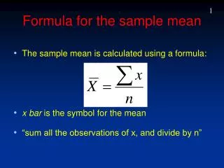
The Sample Mean. 68 - 95 - 99.7 rule. Recall we learned a variable could have a normal distribution.

E N D
68 - 95 - 99.7 rule Recall we learned a variable could have a normal distribution. This was useful because then we could say approximately 68% of the people in the data set have a value on the variable within 1 standard deviation of the mean. Approximately 95% have a value within 2 standard deviations of the mean, and approximately 99.7% have a value within 3 standard deviations of the mean. Let’s look at this idea again in the context of an example. Say we asked a whole bunch of people how many ounces of Mt. Dew they consume each year. Say the responses follow a normal distribution with mean = 5480 and standard deviation = 480.
The rule again 4040 4520 5000 5480 5960 6440 6920 -----68% --- Ounces of Mt. Dew -------------- 95%------------- per year -----------------------------99.7%-----------------------
The rule So, by the rule we know that about 68% of the people in the data set have between 5000 and 5960 ounces of Mt. Dew (ozs of MD)per year. Remember a Z score = (Value – mean)/standard deviation. For example, a person who has 6920 ozs of MD each year has a Z value = (6920 – 5480)/480 = 1440/480 = 3. Similar Z’s are shown for this example on the next slide. Check each calculation! (Don’t say, “yea right man.” Do it )
Z values put below actual values 4040 4520 5000 5480 5960 6440 6920 -3 -2 -1 0 1 2 3 Ounces of Mt. Dew per year
Questions What % of people in the data set had between 5480 and 6920 ozs of MD per year? The Z’s for these two values are 0 and 3, respectively. We saw before how to get the answer. Note Z is carried out to two decimal places. YOU SHOULD ALWAYS CARRY Z OUT TO TWO DECIMAL PLACES! The value we want is .49865
Questions What does .49865 mean? If you were to meet someone at random who was a part of this data set, you would say the probability is .49865 they consume between 5480 and 6920 ozs of MD per year. In other words, 49.865% of the people in the study had between 5480 and 6920 ozs of MD per year. What % of people had between 4040 and 5480 ozs of MD per year? The Z for 4040 is –3. The Z table is symmetric. So the amount between –3 and 0 is the same as between 0 and 3. So 49.865% of the people where between 4040 and 5480.
Questions What % of the people in the study has between 4040 and 6920 ozs of MD per year? The Z’s are –3 and 3. This means you would have people within 3 standard deviations of the mean. You take the amount between –3 and 0 and the amount between 0 and 3. That is 49.865 + 49.865 = 99.73 or close to 99.7%. What % of people had between 4520 and 6440 ozs of MD per year? The Z’s are –2 and 2. From 0 to 2 we have .4772 so the total is .4772 + .4772 = .9544 or 95.44% So within 2 standard deviations is a little more than 95%.
Special Z = 1.96 If you have a Z of 1.96 the value in the table is .9750. So if you are within 1.96 standard deviations of the mean you will have 95% of the people in the data set. Before we said within 2 standard deviations would give you 95% of the people. But to be more precise we only have to be within 1.96 standard deviations to have 95% of the people.
Review Remember back to the normal distribution. We saw we could make probability statements about a range of values for a variable that has a normal distribution as long as we could calculate the Z score or we had access to Excel. Remember to calculate the Z score we need to know the the mean and the standard deviation of the distribution for the variable. We will now find another use for this rule.
Sample Means - overview • We usually take one sample from a population. From the sample we might calculate a sample mean and use the mean to help us understand the population the sample was taken from. • In principle we could take many more samples and calculate means for each sample, but we don’t because it is too time consuming and often expensive.
Sample Means - overview • If we did take more samples we would see all the sample means are not the same and thus the sample statistic has a distribution. • The main point is whether we take more than one sample or not, the statistics we calculate have a distribution. This section helps us understand the sampling distribution of the sample mean.
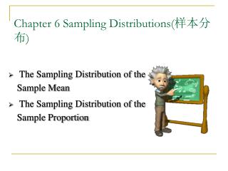
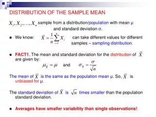
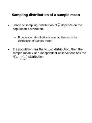
Sample Means - overview • We will see the sampling distribution of the sample mean • 1) is normal • 2) has the same mean as the mean of the population from which the sample is drawn • 3) has a smaller standard deviation than the standard deviation from which the sample was drawn.
Sample Means - The central limit theorem • We really don’t have to worry about the central limit theorem other than the fact that experts(people who live more than 50 miles away) tell us that the sampling distribution of the sample mean is normal.
Sample Means - Mean of sampling distribution population variable mean of population Some samples will have more values from the low side of the mean than other samples. But, overall the mean of the sample means will be right at the population mean.
Sample Means - Standard deviation of sampling distribution • The standard deviation of the sampling distribution is smaller than the standard deviation of the population from which the sample was drawn. • The standard deviation of the sampling distribution equals the standard deviation of the population divided by the square root of the sample size. I need you to accept this fact.
Standard error. The central limit theorem tells us the sampling distribution of sample means has a standard deviation equal to the standard deviation in the population divided by the square root of the sample size by which we draw the sample. A standard deviation is a standard deviation is a standard deviation! When we want to talk about the standard deviation of a sampling distribution we call the standard deviation a standard error. It is a way to make life less complicated (if you know what I mean). So a standard error is a standard deviation, but of a sampling distribution.
Check this out! We have some terminology that is getting somewhat complex. Let’s review some ideas to put it all straight. The population standard deviation of a quantitative variable is a number that suggests how spread out are the data. The sample standard deviation is a point estimate of the population standard deviation. The standard error is the standard deviation of the sampling distribution of the sample mean. Later, we will see we use the population standard deviation or the sample standard deviation to calculate the standard error.
Sampling distributions Statistics like the sample mean have a sampling distribution, in a repeated sampling sense, and thus we can talk about the mean and standard error of the distribution. We know, for example, that 95% of the sample means are within 1.96 standard errors of the population mean. We will build on this concept later.
Some more terminology Say we take a sample and calculate the sample mean age as 35.7. The number 35.7 is called a point estimate of the population mean. We can use one point to estimate the population parameter. The sample mean or average in general says add up all the values and divide by the number of values added. This is a procedure. You talk to 100 people, get their ages, add up their ages and divide by 100. In this sense of being a procedure the sample mean is said to be a point estimator of the population mean. Point estimate – actual value Point estimator - procedure
Let’s say we are told in a population the mean on a variable is 200 and the standard deviation is 50. You would think we could stop and not do any work because we know about the population. But we continue on because we want to illustrate some details. We are told the sample size is 100. From the central limit theorem we know the sampling distribution of the sample mean will be 1. A normal distribution 2. With mean equal to the mean in the population, or 100, 3. With standard error (really just a standard deviation) = 50/sqrt100 = 50/10 = 5 (more on next screen)
In this example what is the probability the sample mean will be within + or – 5 of the population mean? To answer this we must use the sampling distribution of the sample mean. Another way to think of this is what is the probability the sample mean will be between 195 and 205? 195 has the Z = (195 – 200)/5 = -1.00. 205 has Z = 1.00. So the answer is .6828 What is the probability the sample mean will be between 190 and 210. The Z’s are –2 and 2. The answer is .9544