Download
1 / 55
600 likes | 805 Views
The (“Sampling”) Distribution for the Sample Mean*. Distribution of Sample Means. A quantitative population of N units with parameters mean standard deviation A random sample of n units from the population Statistic : The sample mean . Distribution of Sample Means.

E N D
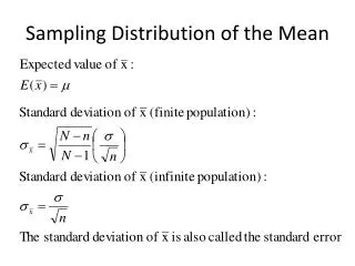
Distribution of Sample Means A quantitative population of N units with parameters mean standard deviation A random sample of n units from the population Statistic: The sample mean .
Distribution of Sample Means Statistic: The sample mean . This statistic is an unbiased point estimate (on average correct) of the parameter.
20 Times Rule / 5% Rule(same thing) If the population size (N) is at least 20 times the sample size (n) N / n 20 or n / N 0.05 then the standard deviation is (essentially)
Distribution of the Sample Mean When the population size is at least 20 times n. Given A variable with population that is not Normally distributed with mean andstandard deviation . A random sample of size n. Result The sample mean has approximate Normal distribution with
Example Rolls of paper leave a factory with weights that are Normal with mean = 1493 lbs, and standard deviation = 12 lbs.
Finding probabilities What is the probability a roll weighs over 1500 lbs? ANS: 0.2798 (about 28% of rolls exceed 1500 lbs)
New Question A truck transports 8 rolls at a time. The legal weight limit for the truck is 12,000 lbs. What is the probability 8 rolls have total weight exceeding this limit? Since 12000/8 = 1500, the question could also be phrased: What is the probability 8 rolls have (sample) mean weight exceeding 1500? The bad news: The answer is not 0.2798. The good news: It’s not that tough.
Review of previous slide Distribution of the Sample Mean Given A variable with population that is Normally distributed with mean andstandard deviation . A random sample of size n. (N/n 20) Result The sample mean has Normal distribution:
Example - continued Rolls (single rolls) of paper leave a factory with weights that are Normal with mean = 1493 lbs, and standard deviation = 12 lbs. If n = 8 rolls are randomly selected, what is the probability their sample mean weight exceeds 1500? The distribution of sample means is Normal.
Finding probabilities Find the probability the sample mean is over 1500 lbs. Here we’re using the same mean, but a standard deviation reduced to 4.243. ANS: 0.0495
The probability the sample mean for 8 rolls exceeds 1500 lbs is 0.0495. For 4.95% of all possible samples of 8 rolls, the sample mean exceeds 1500 lbs. Equivalent: There is a 0.0495 probability that the total weight will exceed 81500 = 12,000 lbs. We’re working towards using the sample mean as an estimate of the population mean. Interpreting the Result
Sample mean weights for samples of 8 rolls. Weights of single rolls. The Picture
About 28% of all rolls are > 1500 lbs The Picture
About 5% of all samples of 8 rolls have mean > 1500 lbs The Picture
Example Survival times have a right skewed distribution with mean = 13 months and standard deviation = 12 months. What can we say about the distribution of sample mean survival times for samples of n patients? As n gets larger, the distribution gets closer to Normal.
Sample mean n = 64SD = 1.5 Single values SD = 12.0 Sample mean n = 16SD = 3.0 Sample mean n = 4SD = 6.0
Distribution of the Sample Mean Assume the population size is at least 20 times n. Given A variable with population that is not Normally distributed with mean andstandard deviation . A random sample of size n. Result The sample mean has approximate Normal distribution with
Distribution of the Sample Mean Given A variable with population that is not Normally distributed with mean andstandard deviation . A random sample of size n. Result The sample mean has generally unknown distribution with
Central Limit Theorem (CLT) Distribution of the Sample Mean Given A variable with population that is not Normally distributed with mean andstandard deviation . A random sample of size n,where n is sufficiently large. Result The sample mean has approximate Normal distribution with
What is “Sufficiently Large?” Your book says “generally n at least 30.” If the population is fairly symmetric without outliers, considerably less than 30 will do the trick. If the population is highly skewed, or not unimodal, considerably more than 30 may be required. If the population is Normal then sample size is not a concern: The sample mean is Normal. You may use the “30” rule if you recognize that it’s not that black and white, and that for Normal populations, n = 1 is “sufficiently large.”
Example The Census Bureau reports the average age at death for female Americans is 79.7 years, with standard deviation 14.5 years. = 79.7 years = 14.5 years What can we say about the distribution of sample means for samples of size 7? It has mean It has standard deviation Is the distribution Normal?
Example Distribution of longevity: 80 15 Within 1 s.d.:
Example Distribution of longevity: 80 15 If Normal Within 1 s.d.: (65, 95)
Example Distribution of longevity: 80 15 If Normal Within 1 s.d.: (65, 95) 68%
Example Distribution of longevity: 80 15 If Normal Within 1 s.d.: (65, 95) 68% Within 2 s.d.s: (50, 110) 95%
Example Distribution of longevity: 80 15 If Normal Within 1 s.d.: (65, 95) 68% Within 2 s.d.s: (50, 110) 95% Above 110
Example Distribution of longevity: 80 15 If Normal Within 1 s.d.: (65, 95) 68% Within 2 s.d.s: (50, 110) 95% Above 110 2.5%
Example Distribution of longevity: 80 15 If Normal Within 1 s.d.: (65, 95) 68% Within 2 s.d.s: (50, 110) 95% Above 110 2.5% 1 in 40 ??? No way! The distribution is not Normal.
Example The Normal shouldn’t be used here (why not?)
Example The Normal shouldn’t be used here (why not?) The distribution of age at death is not Normal. It is quite left skewed. The sample size is not sufficiently large. (At least 30 by your book, although for this situation your instructor would probably buy into as low as 20.) The Central Limit Theorem can’t be applied. The sample mean doesn’t have approximate Normal distribution
Example What can we say about the distribution of sample means for samples of size 7? It has mean It has standard deviation Is the distribution Normal? NO!
Example = 79.7 years = 14.5 years I looked at a few recent obituaries in the Oswego Daily News (online): 79 70 48 99 85 71 45
Example This sample has . A difference of 8.7. Can we compute a Z score for 71.0? Should we? Z = (71.0 – 79.7) /5.48 = 8.7/5.48 = –1.59 Why not? This suggests 71.0 (8.7 from 79.7) is somewhat, but not extremely, unusually low. 71.0 is 1.59 standard deviations from 79.7.
Example Preferred method: Much more compact; faster to work with; essentially identical results. Should we use the Table to obtain probabilities from Z scores (such as our Z = –1.59)? NO If not, how could we get the probabilityof a result within 8.7 from 79.7? Using either a huge database of longevities: Simulate many (all possible) samples of size 7. Determine what proportion of samples give a mean at no more than 8.7 from 79.7. a mathematical model for the longevities Either determine the model for sample means using calculus, or approximate it using numerical methods.
Example What is the distribution of the sample mean of samples of size n = 48? Even though age at death is left skewed, with n = 48 (large enough) the Central Limit Theorem applies, and the sample mean has approximate Normal distribution.
Example I looked at 41 more recent obituaries (total of 48) 79 70 48 99 85 71 45 more data 87 75 90 95 51 99 69 71 49 93 80 89 77 72 101 69 92 92 86 78 92 89 91 81 74 68 89 92 64 71 50 81 88 42 91 44 51 85 81 92 93
Example Median Mean Mode
Example Means for samples of 48 US longevities: Normal My sample The sample mean is (79.7–77.52)=2.18 from the population mean. What is the probability that a random sample of 48 U.S. women’s deaths gives a sample mean at within 2.18 of 79.7. 2.18 below 79.7 is 77.52. 2.18 above 79.7 is 81.88
Example Below 77.52 or above 81.88. Z = 2.18/2.08 = 1.04 Probability = 0.852 – 0.148 = 0.704
Example Find the probability that a random sample of 48 U.S. women’s deaths gives a sample mean at within 2.18 of 79.7. Probability = 0.704 About 30% (that’s almost 1 in 3) of all samples of 48 deaths give a sample mean more than 2.18 from 79.7.
Example Give two explanations that account for the 2.18 year difference between the data on Oswego longevity (which were lower on average) and the U.S. longevity parameter of 79.7. 1. Women in Oswego do not live as long on average as they do nationwide. That is: Oswego< 79.7
Example Give two explanations that account for the 2.18 year difference between the data on Oswego longevity (which were lower on average) and the U.S. longevity parameter of 79.7. 2. Sampling variability (sampling “error”): Oswego= 79.7 About 30% of all samples of 48 women yield a mean 2.18 or more from 79.7. That isn’t so uncommon. Our data aren’t very inconsistent with the national result.
Sampling Without Replacement What to do if the sample size is more than 5% of the population size… N= population size n = sample size N / n 20 n / N ≤ 0.05
Distribution of Sample Means The distribution of the sample mean has > mean (“unbiased”) > standard deviation > shape closer to Normal (but not necessarily Normal)
Word Lengths – Gettysburg Address N = 268 words: Mean length = 4.295. Standard Deviation = 2.123. Not Normal. Right skewed. Can’t use Table A2.
Distribution of Sample Means:n = 5 Sample means from samples of size n = 5 have > mean > standard deviation > shape closer to Normal (but not Normal – a bit right skewed)
The standard deviation of this distribution is 0.942. Distribution of Sample Means : n = 5 The mean of this distribution is 4.295. The shape is close to Normal (but not Normal – there’s right skew).
Distribution of Sample Means : n = 10 Sample means from samples of size n = 10 have > mean > standard deviation > shape closer to Normal (but not exactly Normal – a bit right skewed)
The standard deviation of this distribution is 0.660. Distribution of Sample Means : n = 10 The mean of this distribution is 4.295. The shape is quite close to Normal (just a little right skew – not enough to fuss over).