Download
1 / 24
290 likes | 527 Views
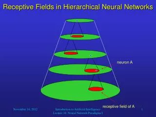
Receptive Fields in Hierarchical Neural Networks. neuron A. receptive field of A. Receptive Fields in Hierarchical Neural Networks. receptive field of A in input layer. neuron A. in top layer. How do NNs and ANNs work?.

E N D
Receptive Fields in Hierarchical Neural Networks neuron A receptive field of A Introduction to Artificial Intelligence Lecture 14: Neural Network Paradigms I
Receptive Fields in Hierarchical Neural Networks receptive field of A in input layer neuron A in top layer Introduction to Artificial Intelligence Lecture 14: Neural Network Paradigms I
How do NNs and ANNs work? • NNs are able to learn by adapting their connectivity patterns so that the organism improves its behavior in terms of reaching certain (evolutionary) goals. • The strength of a connection, or whether it is excitatory or inhibitory, depends on the state of a receiving neuron’s synapses. • The NN achieves learning by appropriately adapting the states of its synapses. Introduction to Artificial Intelligence Lecture 14: Neural Network Paradigms I
An Artificial Neuron synapses neuron i • x1 x2 Wi,1 Wi,2 … xi … Wi,n xn net input signal output Introduction to Artificial Intelligence Lecture 14: Neural Network Paradigms I
The Net Input Signal • The net input signal is the sum of all inputs after passing the synapses: This can be viewed as computing the inner product of the vectors wi and x: where is the angle between the two vectors. Introduction to Artificial Intelligence Lecture 14: Neural Network Paradigms I
fi(neti(t)) 1 0 neti(t) The Activation Function • One possible choice is a threshold function: The graph of this function looks like this: Introduction to Artificial Intelligence Lecture 14: Neural Network Paradigms I
Binary Analogy: Threshold Logic Units Example: w1 = 1 • x1 w2 = 1 x2 = 1.5 x1 x2 x3 w3 = -1 x3 Introduction to Artificial Intelligence Lecture 14: Neural Network Paradigms I
XOR Networks Yet another example: • x1 w1 = = x1 x2 w2 = x2 Impossible! TLUs can only realize linearly separable functions. Introduction to Artificial Intelligence Lecture 14: Neural Network Paradigms I
1 1 1 0 1 1 x2 x2 0 1 0 1 0 0 0 1 0 1 x1 x1 Linear Separability • A function f:{0, 1}n {0, 1} is linearly separable if the space of input vectors yielding 1 can be separated from those yielding 0 by a linear surface (hyperplane) in n dimensions. • Examples (two dimensions): linearly separable linearly inseparable Introduction to Artificial Intelligence Lecture 14: Neural Network Paradigms I
Linear Separability • To explain linear separability, let us consider the function f:Rn {0, 1} with where x1, x2, …, xn represent real numbers. This will also be useful for understanding the computations of artificial neural networks. Introduction to Artificial Intelligence Lecture 14: Neural Network Paradigms I
3 3 3 x2 x2 x2 2 2 2 1 1 1 -3 -3 -3 -2 -2 -2 -1 -1 -1 1 1 1 2 2 2 3 3 3 x1 x1 x1 -1 -1 -1 -2 -2 -2 -3 -3 -3 Linear Separability Input space in the two-dimensional case (n = 2): 1 1 1 0 0 0 w1 = 1, w2 = 2, = 2 w1 = -2, w2 = 1, = 2 w1 = -2, w2 = 1, = 1 Introduction to Artificial Intelligence Lecture 14: Neural Network Paradigms I
Linear Separability • So by varying the weights and the threshold, we can realize any linear separation of the input space into a region that yields output 1, and another region that yields output 0. • As we have seen, a two-dimensional input space can be divided by any straight line. • A three-dimensional input space can be divided by any two-dimensional plane. • In general, an n-dimensional input space can be divided by an (n-1)-dimensional plane or hyperplane. • Of course, for n > 3 this is hard to visualize. Introduction to Artificial Intelligence Lecture 14: Neural Network Paradigms I
x2 1 0 1 0 1 0 0 1 x1 Linear Separability • Of course, the same applies to our original function f using binary input values. • The only difference is the restriction in the input values. • Obviously, we cannot find a straight line to realize the XOR function: In order to realize XOR with TLUs, we need to combine multiple TLUs into a network. Introduction to Artificial Intelligence Lecture 14: Neural Network Paradigms I
Multi-Layered XOR Network 1 • x1 0.5 -1 x2 1 x1 x2 0.5 1 -1 x1 0.5 1 x2 Introduction to Artificial Intelligence Lecture 14: Neural Network Paradigms I
x1 Wi,1 xi Wi,2 x2 Capabilities of Threshold Neurons • What can threshold neurons do for us? • To keep things simple, let us consider such a neuron with two inputs: The computation of this neuron can be described as the inner product of the two-dimensional vectorsx and wi, followed by a threshold operation. Introduction to Artificial Intelligence Lecture 14: Neural Network Paradigms I
second vector component x wi first vector component Capabilities of Threshold Neurons • Let us assume that the threshold = 0 and illustrate the function computed by the neuron for sample vectors wiand x: Since the inner product is positive for -90 90, in this example the neuron’s output is 1 for any input vector x to the right of or on the dotted line, and 0 for any other input vector. Introduction to Artificial Intelligence Lecture 14: Neural Network Paradigms I
Capabilities of Threshold Neurons • By choosing appropriate weights wi and threshold we can place the line dividing the input space into regions of output 0 and output 1in any position and orientation. • Therefore, our threshold neuron can realize any linearly separable function Rn {0, 1}. • Although we only looked at two-dimensional input, our findings apply to any dimensionality n. • For example, for n = 3, our neuron can realize any function that divides the three-dimensional input space along a two-dimension plane. Introduction to Artificial Intelligence Lecture 14: Neural Network Paradigms I
Capabilities of Threshold Neurons • What do we do if we need a more complex function? • Just like Threshold Logic Units, we can also combine multiple artificial neurons to form networks with increased capabilities. • For example, we can build a two-layer network with any number of neurons in the first layer giving input to a single neuron in the second layer. • The neuron in the second layer could, for example, implement an AND function. Introduction to Artificial Intelligence Lecture 14: Neural Network Paradigms I
x1 x1 x1 x2 x2 x2 xi . . . Capabilities of Threshold Neurons • What kind of function can such a network realize? Introduction to Artificial Intelligence Lecture 14: Neural Network Paradigms I
2nd comp. 1st comp. Capabilities of Threshold Neurons • Assume that the dotted lines in the diagram represent the input-dividing lines implemented by the neurons in the first layer: Then, for example, the second-layer neuron could output 1 if the input is within a polygon, and 0 otherwise. Introduction to Artificial Intelligence Lecture 14: Neural Network Paradigms I
Capabilities of Threshold Neurons • However, we still may want to implement functions that are more complex than that. • An obvious idea is to extend our network even further. • Let us build a network that has three layers, with arbitrary numbers of neurons in the first and second layers and one neuron in the third layer. • The first and second layers are completely connected, that is, each neuron in the first layer sends its output to every neuron in the second layer. Introduction to Artificial Intelligence Lecture 14: Neural Network Paradigms I
x1 x1 x1 x2 x2 x2 oi . . . . . . Capabilities of Threshold Neurons • What type of function can a three-layer network realize? Introduction to Artificial Intelligence Lecture 14: Neural Network Paradigms I
2nd comp. 1st comp. Capabilities of Threshold Neurons • Assume that the polygons in the diagram indicate the input regions for which each of the second-layer neurons yields output 1: Then, for example, the third-layer neuron could output 1 if the input is within any of the polygons, and 0 otherwise. Introduction to Artificial Intelligence Lecture 14: Neural Network Paradigms I
Capabilities of Threshold Neurons • The more neurons there are in the first layer, the more vertices can the polygons have. • With a sufficient number of first-layer neurons, the polygons can approximate any given shape. • The more neurons there are in the second layer, the more of these polygons can be combined to form the output function of the network. • With a sufficient number of neurons and appropriate weight vectors wi, a three-layer network of threshold neurons can realize any (!) function Rn {0, 1}. Introduction to Artificial Intelligence Lecture 14: Neural Network Paradigms I