Cortical Receptive Fields Using Deep Autoencoders
Cortical Receptive Fields Using Deep Autoencoders. Work done as a part of CS397 Ankit Awasthi (Y8084) Supervisor: Prof. H. Karnick. The visual pathway. Some Terms.

Cortical Receptive Fields Using Deep Autoencoders
E N D
Presentation Transcript
Cortical Receptive Fields Using Deep Autoencoders Work done as a part of CS397 Ankit Awasthi (Y8084) Supervisor: Prof. H. Karnick
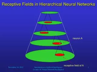
Some Terms • A cell, neuron, neural unit, unit of the neural network may be used interchangeably and all refer to neuron in the visual cortex. • Receptive field of a neuron refers to the region in space in which the presence of a stimulus will change the response of the neuron.
Precortical stages • Retinal cells and the cells in the LGN are center on surround off and vice versa
Why focus on cortical perception?? • Most cells in the precortical stages are hard-coded to a large extent and may be innate • Cortical cells are mostly learned through postnatal visual stimulation • Hubel Wiesel showed that irreversible damage was produced in kittens by sufficient visual deprivation during the so-called critical period
How did you do that?? • Surely you did not use only visual information • Processing in the later stages of visual cortex has some top-down influence • Much of the visual inference involves input from other modalities (say facial emotion recognition) • Thus we focus only on those stages of processing which require/use only visual information
Neurological Findings (with electrodes in cat’s cortex !!) • The visual cortex consists of simple and complex cells • Simple cells can be characterized by a certain distributions of on and off areas • Complex cells could not be explained with a simple distribution of on and off areas • Receptive fields for simple cells should look like oriented edge detectors • Receptive fields of different cells may be overlapping
Topographic Representation • There is a systematic mapping of each structure to the next • The optic fibers from a part of the retina are connected to a small part in LGN • A part of LGN is similarly connected to a small part in the primary visual cortex • This topography continues in other cortical regions • Convergence at each stage Larger receptive fields in later stages
Why Deep Learning?? • Brains have a deep architecture • Humans organize their ideas hierarchically, through composition of simpler ideas • Insufficiently deep architectures can be exponentially inefficient • Deep architectures facilitate feature and sub-feature sharing
Neural Networks (~1985) Compare outputs with correct answer to get error signal Back-propagate error signal to get derivatives for learning outputs hidden layers input vector
Restricted Boltzmann Machines (RBM) • We restrict the connectivity to make learning easier. • Only one layer of hidden units. • No connections between hidden units. • Energy of a joint configuration is defined as • (for binary visible units) • (for real visible units) Hidden(h) j i Visible(v)
Restricted Boltzmann Machines (RBM)(contd.) • Probability of a configuration is defined as • The hidden nodes are conditionally independent given the visible layer and vice versa • Using the definition of the energy function and probability, the conditional probabilities come out to be as follows
Maximum likelihood learning for an RBM j j j j a fantasy i i i i t = 0 t = 1 t = 2 t = infinity Start with a training vector on the visible units. Then alternate between updating all the hidden units in parallel and updating all the visible units in parallel.
Sparse DBNs(Lee at. al. 2007) • In order to have a sparse hidden layer, the average activation of a hidden unit over the training is constrained to a certain small quantity • The optimization problem in the learning algorithm would look like
Related Work • In [4], the authors had shown the features learned by independent component analysis were oriented edge detectors • Lee et. al. in [10] show that the second layer learned using sparse DBNs match certain properties of cells in V2 area of the visual cortex • Bengio et.al. in [3] discuss ways of visualizinng higher layer features • Lee et.al. in [4] have come up with convolutional DBNs which incorporates weight sharing across the visual field and probablistic max pooling operation
Our experimental setting • We trained sparse DBNs on 100,000 randomly sampled patches of natural images of size 14x14 • The image were preprocessed to have same overall contrast and whitened as in [5] • The hidden units in the first, second, third layer are all 200 in number
Getting first layer hidden features • To maximize the activation of the ithhidden unit, the input v should be • Recall what was said about receptive fields of simple cells (oriented edge detectors)
Higher Layer Features • Projecting the a higher layer's weights onto the response of the previous layer…..useless!!! • Three different methods of projecting the hidden units onto the input space • Linear Combination of Previous layer filters, Lee et.al. [2] • Sampling from a hidden unit, Hinton et.al. [5], Bengio et.al.[3] • Activation Maximization, Bengio et.al. [3]
Linear Combination of Previous Layer Filters • Only few connections to the previous layer have their weights either too high or too low • Some of the largest weighted connections are used for linear combination • Overlooks the non-linearity in the network from one layer to the other • Simple and efficient
Sampling from Hidden Units • Deep Autoencoder ( using RBMs ) is a generative model ( top down sampling) and any two adjacent layers form a RBM ( Gibbs sampling) • Clamp a particular hidden unit to 1 during Gibbs sampling and then do a top down sampling to the input layer
Activation Maximization • Intuition same as that for first layer features • Optimization problem is much more difficult • In general a non convex problem • Solve for local minima for different random initializations, then take average or the minimum etc.
Analysis of Results • As observed, the second layer features are able to capture a combination of edges or angled stimuli • The third layer features are very difficult to make sense of in terms of simple geometrical elements • No good characterization of these cells is available, thus not to choose between the different methods
Larger Receptive Fields for Higher Layers We offer a simple solution to extend the size of the receptive fields for higher layers Using the RBM trained on natural image patches, compute the response over the entire image with overlapping patches Responses of some neighboring patches are taken as input for the next layer RBM This is repeated for the whole network This has not been investigated exhaustively
Results(linear combination) First Layer Second Layer
Conclusion and Future Work • Similarities in the receptive fields • Support for Deep Learning Methods as computational model for cortical processing • Able to learn more complete parts of objects in the higher layers with bigger receptive fields • Future work would be to extend these ideas and establish the cognitive relevance of the computational models
References • Georey E. Hinton, Yee-WhyeTeh and Simon Osindero, A Fast Learning Algorithm forDeep Belief Nets. Neural Computation, pages 1527-1554, Volume 18, 2006. • D. H. Hubel & T. N. Wiesel JiroGyoba , Recpetive Fields, Binocular Interaction And Functional Architecture In The Cat's Visual Cortex,The Journal of Physiology, Vol. 16;0, No. 1., 1962 • Michael J. Lyons, Shigeru Akamatsu, Miyuki Kamachi & JiroGyoba , Coding Facial Expressions with Gabor Wavelets,Proceedings, Third IEEE International Conference on Automatic Face and Gesture Recognition,pp 200-205, 1-19.April 14-16 1998 • Hateren, J. H. van and Schaaf, A. van der , Independent Component Filters of Natural Images Compared with Simple Cells in Primary Visual Cortex,Proceedings: Biological Sciences, vol 265,pages 359-366, March 1998 • Georey E. Hinton (2010). A Practical Guide to Training Restricted Boltzmann Machines,TechnicalReport,Volume 1 • DumitruErhan, YoshuaBengio, Aaron Courville, and Pascal Vincent (2010). Visualizing Higher-Layer Features of a Deep Network,Technical Report 1341
References(contd.) • Honglak Lee, Roger Grosse,RajeshRanganath, Andrew Y. Ng. Convolutional Deep Belief Networks for Scalable Unsupervised Learning of Hierarchical Representations,ICML 2009 • Geoffrey E. Hinton Learning multiple layers of representation,Trends in Cognitive Sciences Vol.11 No.10 ,2006 • Andrew Ng. (2010). SparseAutoencoder(lecture notes). • Honglak Lee, ChaitanyaEkanadham, Andrew Y. Ng, Sparse deep belief net model for visual area V2NIPS,2007 • RuslanSalakhutdinov Learning Deep Generative Models Phd thesis, 2009 • YoshuaBengio Learning Deep Architectures for AI Foundations and Trends in Machine Learning,Vol. 2, No. 1, 1127, 2009