Group Analysis
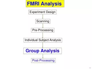
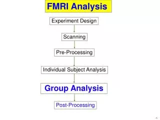
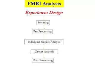
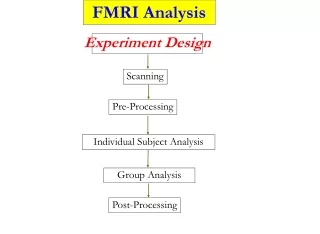
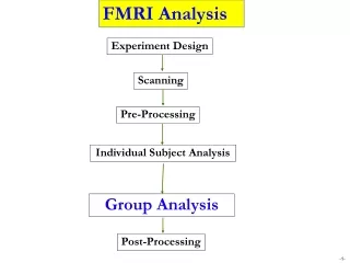
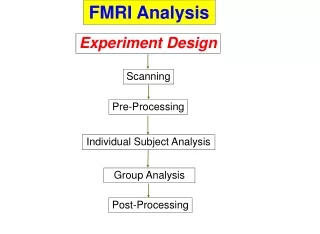
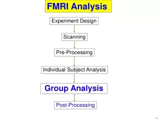
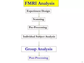
FMRI Analysis. Experiment Design. Scanning. Pre-Processing. Individual Subject Analysis. Group Analysis. Post-Processing. Group Analysis. Basic analysis. Program. Contrasts. Design. 3dttest, 3dANOVA/2/3, 3dRegAna, GroupAna, 3dLME. 3dDeconvolve. Simple Correlation. 3dDecovolve.

Group Analysis
E N D
Presentation Transcript
FMRI Analysis Experiment Design Scanning Pre-Processing Individual Subject Analysis Group Analysis Post-Processing
Group Analysis Basic analysis Program Contrasts Design 3dttest, 3dANOVA/2/3, 3dRegAna, GroupAna, 3dLME 3dDeconvolve Simple Correlation 3dDecovolve Context-Dependent Correlation Connectivity Analysis Path Analysis 1dSEM Causality Analysis 1dVAR
Group Analysis: Why and how? • Group analysis • Make general conclusions about some population, e.g., • Do men and women differ on responding to fear? • What regions are related to happiness, sad, love, faith, empathy, etc.? • What differs when a person listens to classical music vs. rock ‘n’ roll? • Partition/untangle data variability into various effects • Why two tiers of analysis: individual and then group? • No perfect approach to combining both into a batch analysis • Each subject may have slightly different design or missing data • High computation cost • Usually we take β’s (% signal change) to group analysis • Within-subject variation relatively small compared to cross-subject
Group Analysis: Basic concepts • Variables • Dependent: percent signal changes (β’s) • Independent • factors: a categorization (variable) of conditions/tasks/subjects • Covariates (IQ, age) • Fixed factor • Treated as a fixed variable to be estimated in the model • Categorization of experiment conditions (mode: Face/House) • Group of subjects (male/female, normal/patient) • All levels of the factor are of interest and included for replications among subjects • Fixed in the sense of inference • apply only to the specific levels of the factor, e.g., the response to face/house is well-defined • don’t extend to other potential levels that might have been included, e.g., the response to face/house doesn’t say anything about the response to music
Group Analysis: Basic concepts • Random factor • Exclusively refers to subjectin FMRI • Treated as a random variable in the model • random effects uniquely attributable to each subject: N(0, σ2): σ2 to be estimated • Each subject is of NO interest • Random in the sense of inference • subjects serve as a random sample of a population • this is why we recruit a lot of subjects for a study • inferences can be generalized to a population • we usually have to set a long list of criteria when recruiting subjects (right-handed, healthy, age 20-40, native English speaker, etc.) • Covariates • Confounding/nuisance effects • Continuous variables of no interest • May cause spurious effects or decrease power if not modeled • Some measures about subject: age, IQ, cross-conditions/tasks behavior data, etc.
Group Analysis: Types • Fixed: factor, analysis/model/effects • Fixed-effects analysis (sometimes): averaging among a few subjects • Non-parametric tests • Mixed design • Mixed design: crossed [e.g., AXBXC] and nested [e.g., BXC(A)] Psychologists: Within-subject (repeated measures) / between-subjects factor • Mixed-effects analysis (aka random-effects) • ANOVA: contains both types of factors: both inter/intra-subject variances • Crossed, e.g., AXBXC • Nested, e.g., BXC(A) • ANCOVA • LME • Unifying and extending ANOVA and ANCOVA • Using ML or ReML
Group Analysis: What do we get out of the analysis • Using an intuitive example of income (dependent variable) • Factor A: sex (men vs. women) • factor B: race (whites vs. blacks) • Main effect • F: general information about all levels of a factor • Any difference between two sexes or races • men > women; whites > blacks • Is it fair to only focus on main effects? • Interaction • F: Mutual/reciprocal influence among 2 or more factors • Effect of a factor depends on levels of other factors, e.g., • Black men < black women • Black women almost the same as white women • Black men << white men • General linear test • Contrast • General linear test (e.g., trend analysis)
Group Analysis: Types • Averaging across subjects (fixed-effects analysis) • Number of subjects n < 6 • Case study: can’t generalize to whole population • Simple approach (3dcalc) • T = ∑tii/√n • Sophisticated approach • B = ∑(bi/√vi)/∑(1/√vi), T = B∑(1/√vi)/√n, vi = variance for i-thregressor • B = ∑(bi/vi)/∑(1/vi), T = B√[∑(1/vi)] • Combine individual data and then run regression • Mixed-effects analysis • Number of subjects n > 10 • Random effects of subjects • Individual and group analyses: separate • Within-subject variation ignored • Main focus of this talk
Group Analysis: Programs in AFNI • Non-parametric analysis • 4 < number of subjects < 10 • No assumption of normality; statistics based on ranking • Programs • 3dWilcoxon (~ paired t-test) • 3dMannWhitney (~ two-sample t-test) • 3dKruskalWallis (~ between-subjects with 3dANOVA) • 3dFriedman (~one-way within-subject with 3dANOVA2) • Permutation test • Multiple testing correction with FDR (3dFDR) • Less sensitive to outliers (more robust) • Less flexible than parametric tests • Can’t handle complicated designs with more than one fixed factor
Group Analysis: Programs in AFNI • Parametric tests (mixed-effects analysis) • Number of subjects > 10 • Assumption: Gaussian random effects • Programs • 3dttest (one-sample, two-sample and paired t) • 3dANOVA (one-way between-subject) • 3dANOVA2 (one-way within-subject, 2-way between-subjects) • 3dANOVA3 (2-way within-subject and mixed, 3-way between-subjects) • 3dRegAna (regression/correlation, simple unbalanced ANOVA, simple ANCOVA) • GroupAna (Matlab package for up to 5-way ANOVA) • 3dLME (R package for all sorts of group analysis)
Group Analysis: Planning for mixed-effects analysis • How many subjects? • Power/efficiency: proportional to √n; n > 10 • Balance: Equal number of subjects across groups if possible • Input files • Common brain in tlrc space (resolution doesn’t have to be 1x1x1 mm3 ) • Percent signal change (not statistics) or normalized variables • HRF magnitude: Regression coefficients • Linear combinations of β‘s • Analysis design • Number of factors • Number of levels for each factor • Factor types • Fixed (factors of interest) vs. random (subject) • Cross/nesting: Balanced? Within-subject/repeated-measures vs. between-subjects • Which program? • 3dttest, 3dANOVA/2/3, GroupAna, 3dRegAna, 3dLME
Group Analysis: Planning • Thresholding • Two-tail by default in AFNI • If one-tail pis desirable, look for 2p on AFNI • Scripting – 3dANOVA3 • Three-way between-subjects (type 1) • 3 categorizations of groups: sex, disease, age • Two-way within-subject (type 4): Crossed design A×B×C • One group of subjects: 16 subjects • Two categorizations of conditions: A – category; B - affect • Two-way mixed (type 5): B×C(A) • Nesting (between-subjects) factor (A): subject classification, e.g., sex • One category of condition (within-subject factor B): condition (visual vs. auditory) • Nesting: balanced
Model type, Factor levels Input for each cell in ANOVA table: totally 3X3X16 = 144 • Group Analysis: Example – 2-way within-subject ANOVA 3dANOVA3 -type 4 -alevels 3 -blevels 3 -clevels 16 \ -dset 1 1 1 stats.sb04.beta+tlrc’[0]’ \ -dset 1 2 1 stats.sb04.beta+tlrc’[1]’ \ -dset 1 3 1 stats.sb04.beta+tlrc’[2]’ \ -dset 2 1 1 stats.sb04.beta+tlrc’[4]’ \ … -fa Category \ -fb Affect \ -fabCatXAff \ -amean 1 T \ (coding with indices) -acontr 1 0 -1 TvsF\(coding with coefficients) -bcontr 0.5 0.5 -1 non-neu \ (coefficients) -aBcontr 1 -1 0 : 1 TvsE-pos \ (coefficients) -Abcontr 2 : 1 -1 0EPosvsENeg \ (coefficients) -bucket anova33 F tests: Main effects & interaction t tests: 1st order Contrasts t tests: 2nd order Contrasts Output: bundled
Group Analysis: GroupAna • Multi-way ANOVA • Matlab script package for up to 5-way ANOVA • Can handle both volume and surface data • Can handle up to 4-way unbalanced designs • Unbalanced: unequal number of subjects across groups • No missing data from subjects allowed • Downsides • Requires Matlab plus Statistics Toolbox • Slow (minutes to hours): GLM approach - regression through dummy variables • Complicated design, and compromised power • Solution to heavy duty computation • Input with lower resolution recommended • Resample with adwarp -dxyz # or 3dresample • See http://afni.nimh.nih.gov/sscc/gangc for more info • Alternative: 3dLME
Group Analysis: ANCOVA (ANalysis of COVAriances) • Why ANCOVA? • Subjects or cross-regressors effects might not be an ideally randomized • If not controlled, such variability will lead to loss of power and accuracy • Different from amplitude modulation: cross-regressorsvs. within-regressor variation • Direct control via design: balanced selection of subjects (e.g., age group) • Indirect (statistical) control: add covariates in the model • Covariate (variable of no interest): uncontrollable/confounding, usually continuous • Age, IQ, cortex thickness • Behavioral data, e.g., response time, correct/incorrect rate, symptomatology score, … • ANCOVA = Regression + ANOVA • Assumption: linear relation between HDR and the covariate • GLM approach: accommodate both categorical and quantitative variables • Programs • 3dRegAna: for simple ANCOVA • If the analysis can be handled with 3dttest without covariates • See http://afni.nimh.nih.gov/sscc/gangc/ANCOVA.html for more information • 3dLME: R package
Group Analysis: 3dLME • Linear regression vs. Linear mixed-effects (or hierarchical) • R package: Open source platform • Versatile: handles almost all situations in one package • Unbalanced designs (unequal number of subjects, missing data, etc.) • ANOVA and ANCOVA, but unlimited number of factors and covariates • Able to handle HRF modeling with basis functions • Violation of sphericity: heteroscedasticity, variance-covariance structure • Model fine-tuning • No scripting (input is bundled into a text file model.txt) • Disadvantages • High computation cost (lots of repetitive calculation) • Sometimes difficult to compare with traditional ANOVA • See http://afni.nimh.nih.gov/sscc/gangc/lme.html for more information
Group Analysis: 3dLME • Linear (Regression) model • yi = β0+β1x1i + … + βpxpi + εi, εi~ N(0,σ2), for ith subject • Y = Xβ + ε, ε~ Nn(0,σ2Λn), for each subject • Only one random-effect compoent, residual ε • Linear mixed-effects (LME) model • yij = β0+β1x1ij+ … +βpxpij+bi1z1ij+…+biqzqij+εij, bik~N(0,ψk2), cov(bk,bk’)=ψkk’, εij~ N(0,σ2λijj), cov(εij,εij’)= σ2λijj’ • Yi= Xiβ +Zibi+εi, bi~ Nq(0, ψ), εi~ Nni(0,σ2Λi), for ith subject • Two random-effect components: Zibindεi • AN(C)OVA can be incorporated as a special case • ni is constant (>1, repeated-measures), Λi = Inxn(iid)
Group Analysis: 3dLME • Running LME • Create a text file model.txt (3 fixed factors plus 1 covariate) Data:Volume <-- either Volume or Surface Output:FileName<-- any string (no suffix needed) MASK:Mask+tlrc.BRIK <-- mask dataset Model:Age+Gender*Object*Modality <-- model formula for fixed effects COV:Age<-- covariate list RanEff:1 <-- random effects VarStr:0 CorStr:0 Clusters:4 <-- number of parallel jobs SS:sequential MFace-FFace <-- contrast label Male*Face*0*0-Female*Face*0*0 <-- contrast specification MVisual-Maudial Male*0*Visual*0-Male*0*Audial*0 ...... Subj Gender Object Modality Age InputFile Jim Male Face Visual 25 file1+tlrc.BRIK Carol Female House Audial 23 file2+tlrc.BRIK Karl Male House Visual 26 file3+tlrc.BRIK Casey Female Face Audial 24 file4+tlrc.BRIK ...... • Run3dLME.R MyOut &
Group Analysis: 3dLME • HRF modeled with basis functions • Traditional approach: AUC • Hard to detect shape difference • Difficult to handle betas with mixed signs • LME approach • Usually H0:β1=β2=…=βk(not H0: β1=β2=…=βk=0) • But now we don’t care about the differences amongβ’s • Instead we want to detect shape difference • Solution: take allβ’sand model with no intercept • But we have to deal with temporal correlations amongβ’s, Λi ≠ Inxn • For example, AR(1): 2 parameters σ2 and ρfor the residuals
Group Analysis: 3dLME • Running LME: A more complicated example • HRF modeled with 6 tents • Null hypothesis: no HRF difference between two conditions Data:Volume <-- either Volume or Surface Output:test <-- any string (no suffix needed) MASK:Mask+tlrc.BRIK <-- mask dataset Model:Time-1<-- model formula for fixed effects COV: <-- covariate list RanEff:1 <-- random effect specification VarStr:0 <-- heteroscedasticity? CorStr:1~TimeOrder|Subj <-- correlation structure SS: sequential <-- sequential or marginal Clusters:4 <-- number of parallel jobs Subj Time TimeOrderInputFile Jim t1 1 contrastT1+tlrc.BRIK Jim t2 2 contrastT2+tlrc.BRIK Jim t3 3 contrast3+tlrc.BRIK ...... • Output: F for H0, β and t for each basis function
Group Analysis: 3dttest might be your good friend! • Example: 2-way mixed ANOVA with unequal subjects • Can’t use 3dANOVA3 –type 5 • All the t tests can be done with 3dttest • Even main effects and interaction can be obtained for 2×2 design • A: Gender (M vs. F, between-subject); B: stimulus (House vs. Face, within-subject) • Group difference on House: two-sample t-test 3dttest –set1 Male1House … -set2 Female1House … -prefix GroupHDiff • Gender main effect 3dcalc –a Suject1House –b Subject1Face –expr ‘a+b’ –prefix Subject1H+F (Or 3dMean –prefix Subj1CaT Suject1House Subject1Face) 3dttest –set1 Male1H+F … -set2 Female1H+F –prefix HouseEff • Interaction between Gender and Stimulus 3dcalc –a Suject1House –b Subject1Face –expr ‘a-b’ –prefix Subject1HvsF 3dttest –set1 Male1HvsF … -set2 Female1HvsF –prefix Interaction
Group Analysis Basic analysis Program Contrasts Design 3dttest, 3dANOVA/2/3, 3dRegAna, GroupAna, 3dLME 3dDeconvolve Simple Correlation 3dDecovolve Context-Dependent Correlation Connectivity Analysis Path Analysis 1dSEM Causality Analysis 1dVAR
Connectivity: Correlation Analysis • Correlation analysis (aka functional connectivity) • Similarity between a seed region and the rest of the brain • Says not much about causality/directionality • Voxel-wise analysis; Both individual subject and group levels • Two types: simple and context-dependent correlation (a.k.a. PPI) • Steps at individual subject level • Create ROI (a sphere around peak t-statistic or an anatomical structure) • Isolate signal for a condition/task • Extract seed time series • Run correlation analysis through regression analysis • More accurately, partial (multiple) correlation • Steps at group level • Convert correlation coefficients to Z (Fisher transformation): 3dcalc • One-sample t test on Z scores: 3dttest • Interpretation, interpretation, interpretation!!! • Correlation doesn’t mean causation or/and anatomical connectivity • Be careful with group comparison!
Connectivity: Path Analysis or SEM • Causal modeling (a.k.a. structural or effective connectivity) • Start with a network of ROI’s • Path analysis • Assess the network based on correlations (covariances) of ROI’s • Minimize discrepancies between correlations based on data and estimated from model • Input: Model specification, correlation matrix, residual error variances, DF • Output: Path coefficients, various fit indices • Caveats • H0: It is a good model; Accepting H0 is usually desirable • Valid only with the data and model specified • No proof: modeled through correlation analysis • Even with the same data, an alternative model might be equally good or better • If one critical ROI is left out, things may go awry • Interpretation of path coefficient: NOT correlation coefficient, possible >1
Connectivity: Path Analysis or SEM • Path analysis with 1dSEM • Model validation: ‘confirm’ a theoretical model • Null hypothesis: good model! Accept, reject, or modify the model? • Model search: look for ‘best’ model • Start with a minimum model (1): can be empty • Some paths can be excluded (0), and some optional (2) • Model grows by adding one extra path a time • ‘Best’ in terms of various fit criteria • More information http://afni.nimh.nih.gov/sscc/gangc/PathAna.html • Difference between causal and correlation analysis • Predefined network (model-based) vs. network search (data-based) • Modeling: causation (and directionality) vs. correlation • ROI vs. voxel-wise • Input: correlation (condensed) vs. original time series • Group analysis vs. individual + group
Connectivity: Granger Causality or VAR • Causal modeling (a.k.a. structural or effective connectivity) • Start with a network of ROI’s • Causality analysis through vector auto-regressive modeling (VAR) • Assess the network based on correlations of ROIs’ time series • If values of region X provide statistically significant information about future values of Y, X is said to Granger-cause Y • Input: time series from ROIs, covariates (trend, head motion, physiological noise, …) • Output: Path coefficients, various fit indices • Causality analysis with 1dGC • Written in R • Can run both interactive and batch mode • Generate a network and path matrix • A list of model diagnostic tests • Run group analysis on path coefficients • Causality analysis with 3dGC • Seed vs. whole brain
Connectivity: Granger Causality or VAR • Causal modeling (a.k.a. structural or effective connectivity) • Caveats • It has assumptions (stationary property, Gaussian residuals, and linearity) • Require accurate region selection: missing regions may invalidate the analysis • Sensitive to number of lags • Time resolution • No proof: modeled through statistical analysis • Not really cause-effect in strict sense • Interpretation of path coefficient: temporal correlation • SEM versus VAR • Predefined network (model-based) among ROIs • Modeling: statistical causation (and directionality) • Input: correlation (condensed) vs. original time series • Group analysis vs. individual + group
Connectivity: Granger Causality or VAR • Why temporal resolution is important?