FMRI Analysis for Neuroscientific Research
Dive into the basics of fMRI analysis, from experimental design to group analysis, with a focus on Null Hypothesis Significance Testing (NHST) concepts and statistical principles. Learn how to avoid common misinterpretations and enhance the power of your research.

FMRI Analysis for Neuroscientific Research
E N D
Presentation Transcript
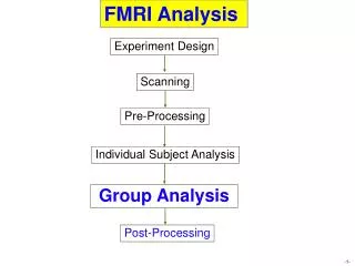
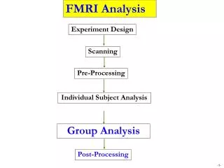
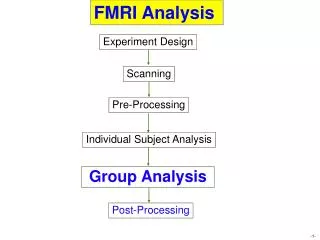
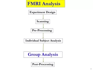
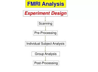
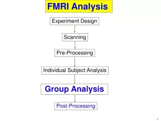
FMRI Analysis Experiment Design Scanning Pre-Processing Individual Subject Analysis Group Analysis Post-Processing
Group Analysis Background Basics ANOVA Program Contrasts Design 3dttest, 3dANOVA/2/3, 3dRegAna Conjunction MTC Cluster Analysis Clusters 3dmerge, 3dclust 3dcalc AlphaSim, 3dFDR
Basics: Null hypothesis significance testing (NHST) • Main function of statistics is to get more information into the data • Null and alternative hypotheses • H0: nothing happened vs. H1: something happened • Dichotomous decision • Rejecting H0 at a significant level α (e.g., 0.05) • Subtle difference Traditional: Hypothesis holds until counterexample occurs; Statistical: discovery holds when a null hypothesis is rejected with some statistical confidence • Topological landscape vs. binary world
Basics: Null hypothesis significance testing (NHST) • Dichotomous decision • Conditional probabilityP( reject H0 | H0) = α ≠ P(H0)! • 2 types of errors and power • Type I error = α = P( reject H0 | H0) • Type II error = β = P( accept H0 | H1) • Power = P( accept H1 | H1) = 1 – β
Basics: Null hypothesis significance testing (NHST) • Compromise and strategy • Lower type II error under fixed type I error • Control false + while gaining as much power as possible • Check efficiency (power) of design with RSFgen before scanning • Typical misinterpretations*) • Reject H0 →Prove or confirm a theory (alternative hypothesis)! (wrong!) • P( reject H0 | H0) = P(H0) (wrong!) • P( reject H0 | H0) = Probability if the experiment can be reproduced (wrong!) *)Cohen, J., "The Earth Is Round (p < .05)” (1994), American Psychologist, 49, 12 997-1003
Basics: Null hypothesis significance testing (NHST) • Controversy: Are humans cognitively good intuitive statisticians? • Quiz: HIV prevalence = 10-3, false + of HIV test = 5%, power of HIV test ~ 100%. • P(HIV+ | test+) = ? • Keep in mind • Better plan than sorry: Spend more time on experiment design (power analysis) • More appropriate for detection than sanctification of a theory • Modern phrenology? • Try to avoid unnecessary overstatement when making conclusions • Present graphics and report % signal change, standard deviation, confidence interval, … • Replications are the best strategy on induction/generalization • Group analysis
QuizA researcher tested the null hypothesis that two population means are equal (H0: μ1 = μ2). A t-test produced p=0.01. Assuming that all assumptions of the test have been satisfied, which of the following statements are true and which are false? Why?1. There is a 1% chance of getting a result even more extreme than the observed one when H0 is true. 2. There is a 1% likelihood that the result happened by chance. 3. There is a 1% chance that the null hypothesis is true. 4. There is a 1% chance that the decision to reject H0 is wrong. 5. There is a 99% chance that the alternative hypothesis is true, given the observed data. 6. A small p value indicates a large effect. 7. Rejection of H0 confirms the alternative hypothesis. 8. Failure to reject H0 means that the two population means are probably equal. 9. Rejecting H0 confirms the quality of the research design. 10. If H0 is not rejected, the study is a failure. 11. If H0 is rejected in Study 1 but not rejected in Study 2, there must be a moderator variable that accounts for the difference between the two studies. 12. There is a 99% chance that a replication study will produce significant results. 13. Assuming H0 is true and the study is repeated many times, 1% of these results will be even more inconsistent with H0 than the observed result.Adapted from Kline, R. B. (2004). Beyond significance testing. Washington, DC: American Psychological Association (pp. 63-69). Dale Berger, CGU 9/04 • Hint: Only 2 statements are true
Basics: Student’s t • Background • Gossett, 1908, Guinness brewing company, Dublin • Named arbitrarily by R. A. Fisher • Bell-shaped, but more spread out • DF: asymptotically approaches N(0,1) as DF→∞ • One tail or two? • Special case of F: t2(n) = F(1, n) • Usages: one-sample, two-sample, and paired t • One-sample • Effect of a condition at group level • Group Mean relative to Standard Error of group Mean (SEM) • Two-sample • Comparison between 2 groups • (Difference of group means)/(Pooled SEM) • Paired • Comparison between 2 conditions at group level • (Difference of conditions)/(SEM of individual differences) • Contrast and general linear test in regression and ANOVA • 3dDeconvolve, 3dRegAna, 3dfim/+, 3dttest, 3dANOVA/2/3 • Assumptions • Gaussian and Sphericity: heteoscedasticity in two-sample t
Basics: F • Background • Named after Sir R. A. Fisher • Ratio of two Chi-square distributions • Two parameters, F(n1, n2) • One tail or two? • t is a special case of F: t2(n) = F(1, n) • Usages: • Two or more samples have the same variance? • ANOVA: Main effects and interactions • What proportion of variation (effect) in the data is attributable to some cause? • Regression: Partial F and glt in 3dRegAna, 3dDeconvolve • Assumptions • Gaussian • Sphericity • More than two conditions • Basis function modeling
Basics: ANOVA • Factor and level • Dependant and independent variable • Factors: categorizing variables, e.g., subject category and stimulus class • Subject categories: sex, genotypes, normal vs. patient • Stimulus categories: 4 (2x2) stimuli, object (human vs. tool), res (motion vs. points) • Levels: nominal (qualitative) values of a factor • Object: human and tool; Resolution: high and low • Fixed/random factor • Fixed: specific levels of a factor are of interest • Random (usually subject in fMRI) • Each level (a specific subject) of the factor is not of interest • But factor variance should be accounted for (cross-subject variation) • Random-effect model • Different terminology for Factorial (crossed)/nested • Count subject as a random factor (statisticians); Random-effect model • Within-subject (repeated measures) / between-subjects (psychologists) • Crossed and nested designs • Group analysis • Make general conclusions about some population • Partition/untangle data variability into various sources (effect → causes)
Basics: ANOVA • More terminology • Main effect: general info regarding all levels of a factor • Simple effect: specific info regarding a factor level • Interaction: mutual/reciprocal influence among 2 or more factors; parallel or not? • Disordinal interaction: differences reverse sign • Ordinal interaction: one above another • Contrast: comparison of 2 or more simple effects; coefficients add up to 0 • General linear test Main effects and interactions in 2-way mixed ANOVA
Group Analysis Background Basics ANOVA Program Contrasts Design 3dttest, 3dANOVA/2/3, 3dRegAna Conjunction MTC Cluster Analysis Clusters 3dmerge, 3dclust 3dcalc AlphaSim, 3dFDR
Group Analysis: Overview • Parametric Tests • 3dttest (one-sample, unpaired and paired t) • 3dANOVA (one-way between-subject) • 3dANOVA2 (one-way within-subject, 2-way between-subjects) • 3dANOVA3 (2-way between-subjects, within-subject and mixed, 3-way between-subjects) • 3dRegAna (regression/correlation, unbalanced ANOVA, ANCOVA) • GroupAna (Matlab script for up to 5-way ANOVA) • Non-Parametric Analysis • No assumption of normality; Statistics based on ranking • Appropriate when number of subjects too few • Programs • 3dWilcoxon (~ paired t-test) • 3dMannWhitney (~ two-sample t-test) • 3dKruskalWallis (~3dANOVA) • 3dFriedman (~3dANOVA2) • Permutation test: plugin on AFNI under Define Datamode / Plugins / • Can’t handle complicated designs • Less sensitive to outliers (more robust) and less flexible than parametric tests
Group Analysis: Overview • How many subjects? • Power: proportional to √n; n > 10 • Efficiency increases by the square root of # subjects • Balance: Equal number of subjects across groups if possible • Input • % signal change (not statistics) • HRF magnitude: Regression coefficients • Contrast • Common brain in tlrc space • Resolution: Doesn’t have to be 1x1x1 mm3 • Design • Number of factors • Number of levels for each factor • Within-subject / repeated-measures vs. between-subjects • Fixed (factors of interest) vs. random (subject) • Nesting: Balanced? • Which program? • Contrasts • One-tail or two-tail?
Group Analysis : 3dttest • Basic usage • One-samplet • One group: simple effect • Example: 15 subjects under condition A with H0:μA= 0 • Two-samplet • Two groups: Compare one group with another • ~ 1-way between-subject (3dANOVA2 -type 1) • Unequal sample sizes allowed • Assumption of equal variance • Example: 15 subjects under A and 13 other subjects under B - H0:μA = μB • Pairedt • Two conditions of one group: Compare one condition with another • ~ one-way within-subject (3dANOVA2 -type 3) • ~ one-sample t on individual contrasts • Example: Difference between conditions A and B for 15 subjects with H0:μA = μB • Output: 2 values (% and t) • Versatile program: Most tests can be done with 3dttest: piecemeal vs. bundled
Group Analysis: 3dANOVA • Generalization of two-sample t-test • One-way between-subject • H0: no difference across all levels (groups) • Examples of groups: gender, age, genotype, disease, etc. • Unequal sample sizes allowed • Assumptions • Normally distributed with equal variances across groups • Results: 2 values (% and t) • 3dANOVA vs. 3dttest • Equivalent with 2 levels (groups) • More than 2 levels (groups): Can run multiple two-sample t-test
Group Analysis: 3dANOVA2 • Designs • One-way within-subject (type 3) • Major usage • Compare conditions in one group • Extension and equivalence of paired t • Two-way between-subjects (type 1) • 1 condition, 2 classifications of subjects • Extension and equivalence two-sample t • Unbalanced designs disallowed: Equal number of subjects across groups • Output • Main effect (-fa): F • Interaction for two-way between-subjects (-fab): F • Contrast testing • Simple effect (-amean) • 1st level (-acontr, -adiff): among factor levels • 2nd level (interaction) for two-way between-subjects • 2 values per contrast: % and t
Group Analysis:3dANOVA3 • Designs • Three-way between-subjects (type 1) • 3 categorizations of groups • Two-way within-subject (type 4): Crossed design AXBXC • Generalization of paired t-test • One group of subjects • Two categorizations of conditions: A and B • Two-way mixed (type 5): Nested design BXC(A) • Two or more groups of subjects (Factor A): subject classification, e.g., gender • One category of condition (Factor B) • Nesting: balanced • Output • Main effect (-fa and -fb) and interaction (-fab): F • Contrast testing • 1st level: -amean, -adiff, -acontr, -bmean, -bdiff, -bcontr • 2nd level: -abmean, -aBdiff, -aBcontr, -Abdiff, -Abcontr • 2 values per contrast : % and t
Group Analysis: GroupAna • Multi-way ANOVA • Matlab script package for up to 5-way ANOVA • Requires Matlab plus Statistics Toolbox • GLM approach (slow) • Powerful: Test for interactions • Downside • Difficult to test and interpret simple effects/contrasts • Complicated design, and compromised power • Heavy duty computation: minutes to hours • Input with lower resolution recommended • Resample with adwarp -dxyz # and 3dresample • Can handle both volume and surface data • Can handle following unbalanced designs (two-sample t type): • 3-way ANOVA type 3: BXC(A) • 4-way ANOVA type 3: BXCXD(A) • 4-way ANOVA type 4: CXD(AXB) • See http://afni.nimh.nih.gov/sscc/gangc for more info
Group Analysis: Example • Design • 4 conditions (TM, TP, HM, HP) and 8 subjects • 2-way within-subject: 2x2x8 • A (Object), 2 levels: Tool vs Human • B (Animation), 2 levels: Motion vs Point • C (subject), 8 levels • AxBxC: Program? 3dANOVA3 -type 4 • Main effects (A and B): 2 F values • Interaction AXB: 1 F • Contrasts • 1st order: TvsH, MvsP • 2nd order: TMvsTP, HMvsHP, TMvsHM, TPvsHP • 6x2 = 12 values • Logistic • Input: 2x2x8 = 32 files (4 from each subject) • Output: 18 subbricks
Model type, number of levels for each factor Input for each cell in ANOVA table: totally 2X2X8 = 32 • Group Analysis: Example • Script 3dANOVA3 -type 4 -alevels 2 -blevels 2 -clevels 8 \ -dset 1 1 1 ED_TM_irf_mean+tlrc \ -dset 1 2 1 ED_TP_irf_mean+tlrc \ -dset 2 1 1 ED_HM_irf_mean+tlrc \ -dset 2 2 1 ED_HP_irf_mean+tlrc \ … -adiff 1 2 TvsH1 \ (indices for difference) -acontr 1 -1 TvsH2 \ (coefficients for contrast) -bdiff 1 2 MvsP1 \ -aBdiff 1 2 : 1 TMvsHM \ (indices for difference) -aBcontr 1 -1 : 1 TMvsHM \ (coefficients for contrast) -aBcontr -1 1 : 2 HPvsTP \ -Abdiff 1 : 1 2 TMvsTP \ -Abcontr 2 : 1 -1 HMvsHP \ -fa ObjEffect \ -fb AnimEffect \ -fab ObjXAnim \ -bucket Group 1st order Contrasts, paired t test 2nd order Contrasts, paired t test Main effects & interaction F test; Equivalent to contrasts Output: bundled
Group Analysis: Example • Alternative approaches • GroupAna • Paired t: 6 tests • Program: 3dttest -paired • For TM vs HM: 16 (2x8) input files (β coefficients: %) from each subject 3dttest -paired -prefix TMvsHM \ -set1 ED_TM_irf_mean+tlrc ... ZS_TM_irf_mean+tlrc \ -set2 ED_HM_irf_mean+tlrc ... ZS_HM_irf_mean+tlrc • One-sample t : 6 tests • Program: 3dttest • For TM vs HM: 8 input files (contrasts: %) from each subject 3dttest -prefix TMvsHM \ -base1 0 \ -set2 ED_TMvsHM_irf_mean+tlrc ... ZS_TMvsHM_irf_mean+tlrc
Group Analysis: ANCOVA • Why ANCOVA? • Subjects might not be an ideally randomized representation of a population • If no controlled, cross-subject variability will lead to loss of power and accuracy • Direct control: balanced selection of subjects • Indirect (statistical) control: untangling covariate effect • Covariate: uncontrollable and confounding variable, usually continuous • Age • Behavioral data, e.g., response time • Cortex thickness • Gender • ANCOVA = Regression + ANOVA • Assumption: linear relation between % signal change and the covariate • GLM approach • Avoid multi-way ANCOVA • Analyze partial data with one-way ANCOVA • Similar to running multiple one-sample or two-sample t test • Centralize covariate so that it would not confound with other effects
Group Analysis: ANCOVA Example • Example: Running ANCOVA • Two groups: 15 normal vs. 13 patients • Analysis: comparing the two groups • Running what test? • Two-sample t with 3dttest • Controlling age effect? • GLM model • Yi = β0 + β1X1i + β2X2i +β3X3i +εi, i = 1, 2, ..., n (n = 28) • Demean covariate (age) X1 • Code the factor (group) with a dummy variable 0, when the subject is a patient; X2i = { 1, when the subject is normal. • With covariate X1 centralized: β0 = effect of patient; β1 = age effect (correlation coef); β2 = effect of normal • X3i= X1i X2i models interaction (optional) between covariate and factor (group) β3 = interaction
Model parameters: 28 subjects, 3 independent variables Memory Input: Covariates, factor levels, interaction, and input files • Group Analysis: ANCOVA Example 3dRegAna -rows 28 -cols 3 \ -workmem 1000 \ -xydata 0.1 0 0 patient/Pat1+tlrc.BRIK \-xydata 7.1 0 0 patient/Pat2+tlrc.BRIK \… -xydata 7.1 0 0 patient/Pat13+tlrc.BRIK \-xydata 2.1 1 2.1 normal/Norm1+tlrc.BRIK \-xydata 2.1 1 2.1 normal/Norm2+tlrc.BRIK \… -xydata -8.9 1 -8.9 normal/Norm14+tlrc.BRIK \-xydata 0.1 1 0.1 normal/Norm15+tlrc.BRIK \ -model 1 2 3 : 0 \ -bucket 0 Pat_vs_Norm \ -brick 0 coef 0 ‘Pat’ \-brick 1 tstat 0 ‘Pat t' \-brick 2 coef 1 'Age Effect' \-brick 3 tstat 1 'Age Effect t' \-brick 4 coef 2 'Norm-Pat' \-brick 5 tstat 2 'Norm-Pat t' \-brick 6 coef 3 'Interaction' \-brick 7 tstat 3 'Interaction t' See http://afni.nimh.nih.gov/sscc/gangc/ANCOVA.html for more information Specify model for F and R2 Output: #subbriks = 2*#coef + F + R2 Label output subbricks
Group Analysis Background Basics Conjunction MTC Cluster Analysis Clusters 3dmerge, 3dclust 3dcalc AlphaSim, 3dFDR ANOVA Program Contrasts Design 3dttest, 3dANOVA/2/3, 3dRegAna
Cluster Analysis: Multiple testing correction • 2 types of errors in statistical tests • What is H0 in FMRI studies? • Type I = P (reject H0|when H0is true) = false positive = p value Type II = P (accept H0|when H1is true) = false negative = β • Usual strategy: controlling type I error (power = 1- β = probability of detecting true activation) • Significance level = α: p < α • Family-Wise Error (FWE) • Birth rate H0: sex ratio at birth = 1:1 • What is the chance there are 5 boys (or girls) in a family? • Among100 families with 5 kids, expected #families with 5 boys =? • In fMRI H0: no activation at a voxel • What is the chance a voxel is mistakenly labeled as activated (false +)? • Multiple testing problem: With n voxels, what is the chance to mistakenly label at least one voxel? Family-Wise Error: αFW = 1-(1- p)n →1 as n increases • Bonferroni correction: αFW = 1-(1- p)n ~ np, if p << 1/n Use p=α/n as individual voxel significance level to achieve αFW = α
Cluster Analysis: Multiple testing correction • Multiple testing problem in fMRI: voxel-wise statistical analysis • Increase of chance at least one detection is wrong in cluster analysis • 3 occurrences of multiple testing: individual, group, and conjunction • Group analysis is the most concerned • Two approaches • Control FWE: αFW = P (≥ one false positive voxel in the whole brain) • Making αFW small but without losing too much power • Bonferroni correction doesn’t work: p=10-8~10-6 *Too stringent and overly conservative: Lose statistical power • Something to rescue? Correlation and structure! *Voxels in the brain are not independent *Structures in the brain • Control false discovery rate (FDR) • FDR = expected proportion of false + voxels among all detected voxels • Concrete example: individual voxel p = 0.001 for a brain of 25,000 EPI voxels • Uncorrected → 25 false + voxels in the brain • FWE: corrected p = 0.05 → 1 false + among 20 brains for a fixed voxel location • FDR: corrected p = 0.05 → 5% voxels in those positively labeled ones are false +
Cluster Analysis: AlphaSim • FWE: Monte Carlo simulations • Named for Monte Carlo, Monaco, where the primary attractions are casinos • Program: AlphaSim • Randomly generate some number (e.g., 1000) of brains with random noise • Count the proportion of voxels are false + in all brains • Parameters: * ROI * Spatial correlation * Connectivity * Individual voxel significant level (uncorrected p) • Output * Simulated (estimated) overall significance level (corrected p-value) * Corresponding minimum cluster size • Decision: Counterbalance among * Uncorrected p • * Minimum cluster size • * Corrected p
Program Restrict correcting region: ROI Spatial correlation • Cluster Analysis: AlphaSim • Example AlphaSim \ -mask MyMask+orig \ -fwhmx 4.5 -fwhmy 4.5 -fwhmz 6.5 \ -rmm 6.3 \ -pthr 0.0001 \ -iter 1000 • Output: 5 columns • Focus on the 1st and last columns, and ignore others • 1st column: minimum cluster size in voxels • Last column: alpha (α), overall significance level (corrected p value) Cl Size Frequency Cum Prop p/Voxel Max Freq Alpha2 1226 0.999152 0.00509459 831 0.859 3 25 0.998382 0.00015946 25 0.137 4 3 1.0 0.00002432 3 0.03 • May have to run several times with different uncorrected p: uncorrected p↑↔ cluster size↑ Connectivity: how clusters are defined Uncorrected p Number of simulations
Cluster Analysis: 3dFDR • Definition: FDR = proportion of false + voxels among all detected voxels • Doesn’t consider • spatial correlation • cluster size • connectivity • Again, only controls the expected % false positives among declared active voxels • Algorithm: statistic (t) p value FDR (q value) z score • Example: 3dFDR -input ‘Group+tlrc[6]' \ -mask_file mask+tlrc \ -cdep -list \ -output test One statistic ROI Arbitrary distribution of p Output
Cluster Analysis: FWE or FDR? Correct type I error in different sense FWE: αFW = P (≥ one false positive voxel in the whole brain) Frequentist’s perspective: Probability among many hypothetical activation brains Used usually for parametric testing FDR = expected % false + voxels among all detected voxels Focus: controlling false + among detected voxels in one brain More frequently used in non-parametric testing Fail to survive correction? At the mercy of reviewers Analysis on surface Tricks One-tail? ROI – cheating? Many factors along the pipeline Experiment design: power? Sensitivity vs specificity Poor spatial alignment among subjects
Cluster Analysis: Conjunction analysis • Conjunction analysis • Common activation area • Exclusive activations • Double/dual thresholding with AFNI GUI • Tricky • Only works for two contrasts • Common but not exclusive areas • Conjunction analysis with 3dcalc • Flexible and versatile • Heaviside unit (step function) defines a On/Off event
Cluster Analysis: Conjunction analysis • Example with 3 contrasts: A vs D, B vs D, and C vs D • Map 3 contrasts to 3 numbers: A > D: 1; B > D: 2; C > D: 4 (why 4?) • Create a mask with 3 subbricks of t (all with a threshold of 4.2) 3dcalc -a func+tlrc'[5]' -b func+tlrc'[10]' -c func+tlrc'[15]‘ \ -expr 'step(a-4.2)+2*step(b-4.2)+4*step(c-4.2)' \ -prefix ConjAna • 8 (=23) scenarios: 0: none; 1: A > D but no others; 2: B > D but no others; 3: A > D and B > D but not C > D; 4: C > D but no others; 5: A > D and C > D but not B > D; 6: B > D and C > D but not A > D; 7: A > D, B > D and C > D
Miscellaneous • Fixed-effects analysis • Sphericity and Heteroscedasticity • Trend analysis • Correlation analysis (aka functional connectivity)
Need Help? Command with “-help” 3dANOVA3 -help Manuals http://afni.nimh.nih.gov/afni/doc/manual/ Web http://afni.nimh.nih.gov/sscc/gangc Examples: HowTo#5 http://afni.nimh.nih.gov/afni/doc/howto/ Message board http://afni.nimh.nih.gov/afni/community/board/ Appointment Contact us @1-800-NIH-AFNI