Group Analysis
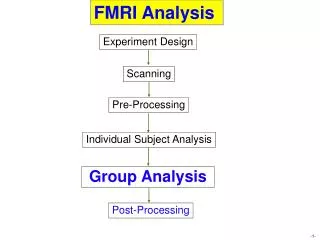
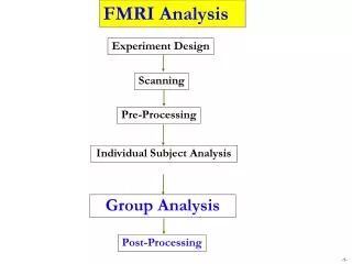
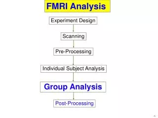
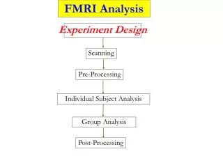
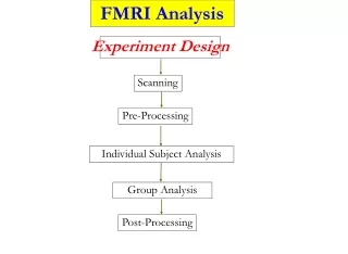
FMRI Analysis. Experiment Design. Scanning. Pre-Processing. Individual Subject Analysis. Group Analysis. Post-Processing. Group Analysis. Basic analysis. Program. Contrasts. Design. 3dttest, 3dANOVA/2/3, 3dRegAna, GroupAna, 3dLME. Conjunction. Cluster Analysis. MTC. Clusters.


Group Analysis
E N D
Presentation Transcript
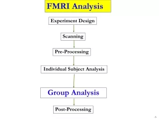
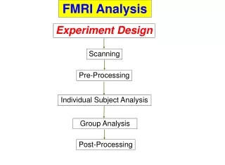
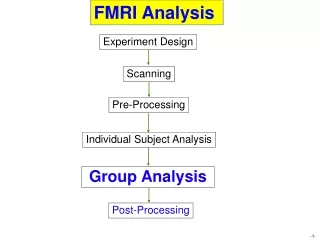
FMRI Analysis Experiment Design Scanning Pre-Processing Individual Subject Analysis Group Analysis Post-Processing
Group Analysis Basic analysis Program Contrasts Design 3dttest, 3dANOVA/2/3, 3dRegAna, GroupAna, 3dLME Conjunction Cluster Analysis MTC Clusters 3dmerge, 3dclust 3dcalc AlphaSim, 3dFDR Simple Correlation Connectivity Analysis Context-Dependent Correlation Path Analysis
Group Analysis: Basic concepts • Group analysis • Make general conclusions about some population • Partition/untangle data variability into various sources • Why two ties of analysis? • High computation cost • Within-subject variation ignored • Mess in terminology • Fixed: factor, model (effects) • Fixed-effects analysis (sometimes): averaging a few subjects • Random: factor, model (effects) • Random-effects analysis (sometimes): subject as a random factor But really a mixed-effects analysis • Psychologists: Within-subject (repeated measures) / between-subjects factor • Mixed: design, model (effects) • Mixed design: crossed [e.g., AXBXC] and nested [e.g., BXC(A)] • Mixed-effects: model with both types of factors; model with both inter/intra-subject variances
Group Analysis: Basic concepts • Fixed factor • Treated as a fixed variable in the model • Categorization of experiment conditions (modality: visual/audial) • Group of subjects (gender, normal/patients) • All levels of the factor are of interest and included for all replications • Fixed in the sense inferences • apply only to the specific levels of the factor • don’t extend to other potential levels that might have been included • Random factor • Exclusively subject in FMRI • Treated as a random variable in the model • average + effects uniquely attributable to each subject: N(μ, σ2) • Each subject is of NO interest • Random in the sense • subjects serve as a random sample of a population • inferences can be generalized to a population
Group Analysis: Types • Averaging across subjects • Number of subjects n < 6 • Case study: can’t generalize to whole population • Simple approach (3dcalc) • T = ∑tii/√n • Sophisticated approach • B = ∑(bi/√vi)/∑(1/√vi), T = B∑(1/√vi)/√n, vi = variance for i-th regressor • B = ∑(bi/vi)/∑(1/vi), T = B√[∑(1/vi)] • Combine individual data and then run regression • Mixed-effects analysis • Number of subjects n > 10 • Random effects of subjects • Individual and group analyses: separate • Within-subject variation ignored • Main focus of this talk
Group Analysis: Programs in AFNI • Non-parametric analysis • 4 < number of subjects < 10 • No assumption of normality; statistics based on ranking • Programs • 3dWilcoxon (~ paired t-test) • 3dMannWhitney (~ two-sample t-test) • 3dKruskalWallis (~ between-subjects with 3dANOVA) • 3dFriedman (~one-way within-subject with 3dANOVA2) • Permutation test: plugin on AFNI under Define Datamode / Plugins /; C program by Tom Holroyd • Multiple testing correction with FDR (3dFDR) • Can’t handle complicated designs • Less sensitive to outliers (more robust) and less flexible than parametric tests
Group Analysis: Programs in AFNI • Parametric tests • Number of subjects > 10 • Assumption: Gaussian • Programs • 3dttest (one-sample, two-sample and paired t) • 3dANOVA (one-way between-subject) • 3dANOVA2 (one-way within-subject, 2-way between-subjects) • 3dANOVA3 (2-way within-subject and mixed, 3-way between-subjects) • 3dRegAna (regression/correlation, hi-way or unbalanced ANOVA, ANCOVA) • GroupAna (Matlab package for up to 5-way ANOVA) • 3dLME (R package for all sorts of group analysis)
Group Analysis: Planning • How many subjects? • Power/efficiency: proportional to √n; n > 10 • Balance: Equal number of subjects across groups if possible • Input files • Common brain in tlrc space (resolution doesn’t have to be 1x1x1 mm3 ) • % signal change (not statistics) or normalized variables • HRF magnitude: Regression coefficients • Contrasts • Design • Number of factors • Number of levels for each factor • Factor types • Fixed (factors of interest) vs. random (subject) • Cross/nesting: Balanced? Within-subject/repeated-measures vs. between-subjects • Which program? • 3dttest, 3dANOVA/2/3, GroupAna, 3dLME
Group Analysis: Planning • Output • Main effect F • F: general information about all levels of a factor • Any difference response between two sexes • Interaction F • Mutual/reciprocal influence among 2 or more factors • Effect for each factor depends on levels of other factors • Example • Dependent variable: income • Factor A: sex (men vs. women); factor B: race (whites vs. blacks) • Main effects: men > women; whites > blacks • Is it fair to only focus on main effects? Interaction! Black men < black women; Black women almost the same as white women; Black men << white men
Group Analysis: Planning • Output • General linear test • Contrast • General linear test • Trend analysis • Thresholding • Two-tail by default • For a desirable one-tail p, look for 2p on AFNI • Scripting – 3dANOVA3 • Three-way between-subjects (type 1) • 3 categorizations of groups: sex, disease, age • Two-way within-subject (type 4): Crossed design AXBXC • One group of subjects: 16 subjects • Two categorizations of conditions: A – category; B - affect • Two-way mixed (type 5): BXC(A) • Nesting (between-subjects) factor (A): subject classification, e.g., sex • One category of condition (within-subject factor B): condition (visual vs. audial) • Nesting: balanced
Model type, Factor levels Input for each cell in ANOVA table: totally 3X3X8 = 32 • Group Analysis: Example 3dANOVA3 -type 4 -alevels 3 -blevels 3 -clevels 16 \ -dset 1 1 1 stats.sb04.beta+tlrc’[0]’ \ -dset 1 2 1 stats.sb04.beta+tlrc’[1]’ \ -dset 1 3 1 stats.sb04.beta+tlrc’[2]’ \ -dset 2 1 1 stats.sb04.beta+tlrc’[4]’ \ … -fa Category \ -fb Affect \ -fab CatXAff \ -amean 1 T \ (coding with indices) -adiff 1 2 TvsE \ (coding with indices) -acontr 1 0 -1 TvsF \ (coding with coefficients) -bcontr 0.5 0.5 -1 non-neu \ (coefficients) -aBdiff 1 2 : 1 TvsE-pos \ (indices) -aBcontr 1 -1 0 : 1 TvsE-pos \ (coefficients) -Abdiff 1 : 1 2 TMvsTP \ (indices) -Abcontr 2 : 1 -1 0 HMvsHP \ (coefficients) -bucket anova33 F tests: Main effects & interaction F tests: 1st order Contrasts F tests: 2nd order Contrasts Output: bundled
Group Analysis: GroupAna • Multi-way ANOVA • Matlab script package for up to 5-way ANOVA • Can handle both volume and surface data • Can handle up to 4-way unbalanced designs • No missing data allowed • Downsides • Requires Matlab plus Statistics Toolbox • GLM approach: regression through dummy variables • Complicated design, and compromised power • Heavy duty computation • minutes to hours • Input with lower resolution recommended • Resample with adwarp -dxyz # or 3dresample • See http://afni.nimh.nih.gov/sscc/gangc for more info • Alternative: 3dLME
Group Analysis: ANCOVA (ANalysis of COVAriances) • Why ANCOVA? • Subjects might not be an ideally randomized representation of a population • If not controlled, cross-subject variability will lead to loss of power and accuracy • Different from amplitude modulation: cross-subject vs. within-subject variation • Direct control through experiment design: balanced selection of subjects (e.g., age group) • Indirect (statistical) control: add covariates in the model • Covariate (variable of no interest): uncontrollable/confounding, usually continuous • Age, IQ, cortex thickness • Behavioral data, e.g., response time, correct rate, symptomatology score, … • Even categorical factors such as gender • ANCOVA = Regression + ANOVA • Assumption: linear relation between HDR and the covariate • GLM approach: accommodate both categorical and quantitative variables • Programs • 3dRegAna: for simple ANCOVA • If the analysis can be handled with 3dttest without covariates • 3dLME: R package (versatile)
Group Analysis: ANCOVA Example • Example: Running ANCOVA • Two groups: 15 normal vs. 13 patients • Analysis • Compare two group: without covariates, two-sample t with 3dttest • Controlling age effect • GLM model • Yi = β0 + β1X1i + β2X2i +β3X3i +εi, i = 1, 2, ..., n (n = 28) • Code the factor (group) with dummy coding 0, when the subject is a patient – control group; X2i = { 1, when the subject is normal. • Centralize covariate (age) X1 so that β0 = patient effect; β1 = age effect (correlation coef); β2 = normal vs patient • X3i= X1i X2i models interaction (optional) between covariate and factor (group) β3 = interaction
Model parameters: 28 subjects, 3 independent variables Input: Covariates, factor levels, interaction, and input files • Group Analysis: ANCOVA Example 3dRegAna -rows 28 -cols 3 \ -xydata 0.1 0 0 patient/Pat1+tlrc.BRIK \-xydata 7.1 0 0 patient/Pat2+tlrc.BRIK \… -xydata 7.1 0 0 patient/Pat13+tlrc.BRIK \-xydata 2.1 1 2.1 normal/Norm1+tlrc.BRIK \-xydata 2.1 1 2.1 normal/Norm2+tlrc.BRIK \…-xydata 0.1 1 0.1 normal/Norm15+tlrc.BRIK \ -model 1 2 3 : 0 \ -bucket 0 Pat_vs_Norm \ -brick 0 coef 0 ‘Pat’ \-brick 1 tstat 0 ‘Pat t' \-brick 2 coef 1 'Age Effect' \-brick 3 tstat 1 'Age Effect t' \-brick 4 coef 2 'Norm-Pat' \-brick 5 tstat 2 'Norm-Pat t' \-brick 6 coef 3 'Interaction' \-brick 7 tstat 3 'Interaction t' See http://afni.nimh.nih.gov/sscc/gangc/ANCOVA.html for more information Specify model for F and R2 Output: #subbriks = 2*#coef + F + R2 Label output subbricks for β0,β1,β2,β3
Group Analysis: 3dLME • An R package • Open source platform • Linear mixed-effects modeling (LME) • Handles various situations in one package • Unbalanced designs • Missing data • ANOVA and ANCOVA • Modeling with basis functions • Heteroscedasticity, variance-covariance structure • Disadvantages • High computation cost • Sometimes difficult to compare with traditional ANOVA • Still under development • See http://afni.nimh.nih.gov/sscc/gangc/lme.html for more information
Group Analysis Basic analysis Program Contrasts Design 3dttest, 3dANOVA/2/3, 3dRegAna, GroupAna, 3dLME Conjunction Cluster Analysis MTC Clusters 3dmerge, 3dclust 3dcalc AlphaSim, 3dFDR Simple Correlation Connectivity Analysis Context-Dependent Correlation Path Analysis
Cluster Analysis: Multiple testing correction • Two types of errors • What is H0 in FMRI studies? H0: no activation at a voxel • Type I = P (reject H0|when H0is true) = false positive = p value Type II = P (accept H0|when H1is true) = false negative = β power = 1- β = probability of detecting true activation • Strategy: controlling type I error while increasing power (decreasing type II) • Significance level α(magic number 0.05) : p < α • Family-Wise Error (FWE) • Birth rate H0: sex ratio at birth = 1:1 • What is the chance there are 5 boys (or girls) in a family? (1/2)5 ~ 0.03 • In a pool of 10000 families with 5 kids, expected #families with 5 boys =? 10000X(2)5 ~ 300 • Multiple testing problem: voxel-wise statistical analysis • With n voxels, what is the chance to mistake ≥ one voxel? Family-Wise Error: αFW = 1-(1- p)n →1 as n increases • n ~ 20,000 voxels in the brain
Cluster Analysis: Multiple testing correction • Multiple testing problem in FMRI • 3 occurrences of multiple tests: individual, group, and conjunction • Group analysis is the most concerned • Approaches • Control FWE • Overall significance: αFW = P (≥ one false positive voxel in the whole brain) • Bonferroni correction: αFW = 1-(1- p)n ~ np, if p << 1/n * Use p=α/n as individual voxel significance level to achieve αFW = α * Too stringent and overly conservative: p=10-8~10-6 • Something to rescue? * Correlation: Voxels in the brain are not independent * Cluster: Structures in the brain * Control FWE based on spatial correlation and cluster size • Control false discovery rate (FDR) • FDR = expected proportion of false + voxels among all detected voxels
Cluster Analysis: AlphaSim • FWE in AFNI • Monte Carlo simulations with AlphaSim • Named for Monte Carlo, Monaco, where the primary attractions are casinos • Program: AlphaSim • Randomly generate some number (e.g., 1000) of brains with white noise • Count the proportion of voxels are false + in ALL (e.g., 1000) brains • Parameters: * ROI - mask * Spatial correlation - FWHM * Connectivity – radium: how to identify voxels belong to a cluster? * Individual voxel significant level - uncorrected p • Output * Simulated (estimated) overall significance level (corrected p-value) * Corresponding minimum cluster size
Program Restrict correcting region: ROI Spatial correlation • Cluster Analysis: AlphaSim • Program: AlphaSim • See detailed steps at http://afni.nimh.nih.gov/sscc/gangc/mcc.html • Example • AlphaSim \ • -mask MyMask+orig \ • -fwhmx 8.5 -fwhmy 7.5 -fwhmz 8.2 \ • -rmm 6.3 \ • -pthr 0.0001 \ • -iter 1000 • Output: 5 columns * Focus on the 1st and last columns, and ignore others * 1st column: minimum cluster size in voxels * Last column: alpha (α), overall significance level (corrected p value) Cl Size Frequency Cum Prop p/Voxel Max Freq Alpha2 1226 0.999152 0.00509459 831 0.859 5 25 0.998382 0.00015946 25 0.137 10 3 1.0 0.00002432 3 0.03 • May have to run several times with different uncorrected p uncorrected p↑↔ cluster size↑ Connectivity: how clusters are defined Uncorrected p Number of simulations
Cluster Analysis: 3dFDR • Definition FDR = % false + voxels among all detected voxels in ONE brain • FDR only focuses on individual voxel’s significance level within the ROI, but doesn’t consider any spatial structure • spatial correlation • cluster size • Algorithm • statistic (t) p value FDR (q value) z score • Example 3dFDR -input ‘Group+tlrc[6]' \ -mask_file mask+tlrc \ -cdep -list \ -output test One statistic ROI Arbitrary distribution of p Output
Cluster Analysis: FWE or FDR? FWE or FDR? Correct type I error in different sense FWE: αFW = P (≥ one false positive voxel in the whole brain) Frequentist’s perspective: Probability among many hypothetical activation brains Used usually for parametric testing FDR = expected % false + voxels among all detected voxels Focus: controlling false + among detected voxels in one brain More frequently used in non-parametric testing Concrete example Individual voxel p = 0.001 for a brain of 25,000 EPI voxels Uncorrected → 25 false + voxels in the brain FWE: corrected p = 0.05 → 5% false + hypothetical brains for a fixed voxel location FDR: corrected p = 0.05 → 5% voxels in those positively labeled ones are false + Fail to survive correction? Tricks One-tail? ROI – e.g., grey matter or whatever ROI you planned to look into Analysis on surface
Cluster Analysis: Conjunction analysis • Conjunction analysis • Common activation area: intersection • Exclusive activations • With n entities, we have 2n possibilities (review your combinatorics!) • Tool: 3dcalc • Heaviside unit (step function) defines a On/Off event
Cluster Analysis: Conjunction analysis • Example • 3 contrasts A, B, and C • Assign each based on binary system: A: 001(20=1); B: 010(21=2); C: 100(22=4) • Create a mask with 3 sub-bricks of t (e.g., threshold = 4.2) 3dcalc -a ContrA+tlrc -b ContrB+tlrc -c ContrC+tlrc \ -expr ‘1*step(a-4.2)+2*step(b-4.2)+4*step(c-4.2)' \ -prefix ConjAna • Interpret output - 8 (=23) scenarios: 000(0): none; 001(1): A but no others; 010(2): B but no others; 011(3): A and B but not C; 100(4): C but no others; 101(5): A and C but not B; 110(6): B and C but not A; 111(7): A, B and C
Cluster Analysis: Conjunction analysis • Multiple testing correction issue • How to calculate the p-value for the conjunction map? • No problem if each entity was corrected before conjunction analysis • But that may be too stringent and over-corrected • With 2 or 3 entities, analytical calculation possible • Each can have different uncorrected p • Double or triple integral of Gaussian distribution • With more than 3 entities, may have to resort to simulations • Monte Carlo simulations • A program in the pipeline?
Group Analysis Basic analysis Program Contrasts Design 3dttest, 3dANOVA/2/3, 3dRegAna, GroupAna, 3dLME Conjunction Cluster Analysis MTC Clusters 3dmerge, 3dclust 3dcalc AlphaSim, 3dFDR Simple Correlation Connectivity Analysis Context-Dependent Correlation Path Analysis
Connectivity: Correlation Analysis • Correlation analysis (a.k.a. functional connectivity) • Similarity between a seed region and the rest of the brain • Says nothing about causality/directionality • Voxel-wise analysis • Both individual subject and group levels • Two types: simple and context-dependent correlation (a.k.a. PPI) • Steps at individual subject level • Create ROI • Isolate signal for a condition/task • Extract seed time series • Correlation analysis through regression analysis • More accurately, partial (multiple) correlation • Steps at group level • Convert correlation coefficients to Z (Fisher transformation): 3dcalc • One-sample t test on Z scores: 3dttest • More details: http://afni.nimh.nih.gov/sscc/gangc
Connectivity: Path Analysis or SEM • Causal modeling (a.k.a. structural connectivity) • Start with a network of ROI’s • Path analysis • Assess the network based on correlations (covariances) of ROI’s • Minimize discrepancies between correlations based on data and estimated from model • Input: Model specification, correlation matrix, residual error variances, DF • Output: Path coefficients, various fit indices • Caveats • Valid only with the data and model specified • No proof: modeled through correlation (covariance) analysis • Even with the same data, an alternative model might be equally good or better • If one critical ROI is left out, things may go awry
Connectivity: Path Analysis or SEM • Path analysis with 1dSEM • Model validation: ‘confirm’ a theoretical model • Accept, reject, or modify the model? • Model search: look for ‘best’ model • Start with a minimum model (can be empty) • Some paths can be excluded • Model grows by adding one extra path a time • ‘Best’ in terms of various fit criteria • More information http://afni.nimh.nih.gov/sscc/gangc/PathAna.html • Difference between causal and correlation analysis • Predefined network (model-based) vs. network search (data-based) • Modeling: causation (and directionality) vs. correlation • ROI vs. voxel-wise • Input: correlation (covariance) vs. original time series • Group analysis vs. individual + group