Download

1 / 37
380 likes | 605 Views
Maps in the Brain – Introduction. Cortical Maps. Cortical Maps map the environment onto the brain. This includes sensory input as well as motor and mental activity. Example: Map of sensory and motor representations of the body (homunculus).The more important a region, the bigger its

E N D
Cortical Maps Cortical Maps map the environment onto the brain. This includes sensory input as well as motor and mental activity. Example: Map of sensory and motor representations of the body (homunculus).The more important a region, the bigger its map representation. Scaled “remapping” to real space
y y x x Place Field Recordings Terrain: 40x40cm Single cell firing activity • Map firing activity to position within terrain • Place cell is only firing around a certain position (red area) • Cell is like a “Position Detector”
Place cells Visual Olfactory Auditory Taste Somatosensory Self-motion Hippocampus • Hippocampus involved in learning and memory • All sensory input into hippocampus • Place cells in hippocampus get all sensory information • Information processing via trisynaptic loop • How place are exactly used for navigation is unknown
Mathematics of the model • Firing rate r of Place Cell i at time t is modeled as Gaussian function: σf is width of the Gaussian function, X and W are vectors of length n, ||* || is theeuclidean distance • At every time step only on weight W is changed (Winner-Takes-All), i.e. the neuron with the strongest response is changed:
Cortical Mapping retinal (x,y) to log Z Coordinates On „Invariance“ A majorproblemishowthebraincanrecognizeobject in spiteofsizeandrotationchanges! Real Space log Z Space ConcentricCirclesVertical Lines (expon. Spaced) (equallyspaced) Radial Lines Horizontal Lines (equalangular spacing) (equallyspaced) Scalingand Rotation defined in Polar Coordinates: Scaling A = k r exp(if) = k a a = r exp(if) Scalingconstant Rotation A = exp(ig) r exp(if) = r exp(i[f+g]) = a exp(ig) Rotation angle After log Z transformweget: Scaling: log(ka) = log(k) + log(a) Rotation: log(a exp(ig)) = ig + log(a) Thus wehaveobtainedscaleandrotationinvariance !
Receptive fields Cells in the visual cortex have receptive fields (RF). These cells react when a stimulus is presented to a certain area on the retina, i.e. the RF. Simple cells react to an illuminated bar in their RF, but they are sensitive to its orientation (see classical results of Hubel and Wiesel, 1959). Bars of different length are presented with the RF of a simple cell for a certain time (black bar on top). The cell's response is sensitive to the orientation of the bar.
2d Map Colormap of preferred orientation in the visual cortex of a cat. One dimensional experiments like in the previous slide correspond to an electrode trace indicated by the black arrow. Small white arrows are VERTICES where all orientations meet.
Ocular Dominance Columns The signals from the left and the right eye remain separated in the LGN. From there they are projected to the primary visual cortex where the cells can either be dominated by one eye (ocular dominance L/R) or have equal input (binocular cells).
Ocular Dominance Columns The signals from the left and the right eye remain separated in the LGN. From there they are projected to the primary visual cortex where the cells can either be dominated by one eye (ocular dominance L/R) or have equal input (binocular cells). White stripes indicate left and black stripes right ocular dominance (coloring with desoxyglucose).
Ice Cube Model Columns with orthogonal directions for ocularity and orientation. Hubel and Wiesel, J. of Comp. Neurol., 1972
Ice Cube Model Columns with orthogonal directions for ocularity and orientation. Problem: Cannot explain the reversal of the preferred orientation changes and areas of smooth transitions are overestimated (see data). Hubel and Wiesel, J. of Comp. Neurol., 1972
Graphical Models Preferred orientations are identical to the tangents of the circles/lines. Both depicted models are equivalent. Vortex: All possible directions meet at one point, the vortex. Problem: In these models vortices are of order 1, i.e. all directions meet in one point, but 0° and 180° are indistinguishable. Braitenberg and Braitenberg, Biol.Cybern., 1979
Graphical Models Preferred orientations are identical to the tangents of the circles/lines. Both depicted models are equivalent. Vortex: All possible directions meet at one point, the vortex. Problem: In these models vortices are of order 1, i.e. all directions meet in one point, but 0° and 180° are indistinguishable. From data: Vortex of order 1/2. Braitenberg and Braitenberg, Biol.Cybern., 1979
Graphical Models cont'd In this model all vertices are of order 1/2, or more precise -1/2 (d-blob) and +1/2 (l-blob). Positive values mean that the preferred orientation changes in the same way as the path around the vertex and negative values mean that they change in the opposite way. Götz, Biol.Cybern., 1988
Developmental Models Start from an equal orientation distribution and develop a map by ways of a developmental algorithm. Are therefore related to learning and self-organization methods.
Model based on differences in On-Off responses KD Miller, J Neurosci. 1994
Resulting receptive fields Resulting orientation map Difference Corre- lation Function
Learning Synaptic Modifications
Structure of a Neuron: At the dendrite the incoming signals arrive (incoming currents) At the soma current are finally integrated. At the axon hillock action potential are generated if the potential crosses the membrane threshold The axon transmits (transports) the action potential to distant sites CNS Systems At the synapses are the outgoing signals transmitted onto the dendrites of the target neurons Areas Local Nets Neurons Synapses Molekules
Chemical synapse:Learning = Change of Synaptic Strength Neurotransmitter Receptors
Different Types/Classes of Learning • Unsupervised Learning (non-evaluative feedback) • Trial and Error Learning. • No Error Signal. • No influence from a Teacher, Correlation evaluation only. • Reinforcement Learning (evaluative feedback) • (Classic. & Instrumental) Conditioning, Reward-based Lng. • “Good-Bad” Error Signals. • Teacher defines what is good and what is bad. • Supervised Learning (evaluative error-signal feedback) • Teaching, Coaching, Imitation Learning, Lng. from examples and more. • Rigorous Error Signals. • Direct influence from a teacher/teaching signal.
dwi = m ui v m << 1 Basic Hebb-Rule: dt A reinforcement learning rule (TD-learning): One input, one output, one reward. A supervised learning rule (Delta Rule): No input, No output, one Error Function Derivative, where the error function compares input- with output- examples. An unsupervised learning rule: For Learning: One input, one output.
Self-organizing maps:unsupervised learning input map Neighborhood relationships are usually preserved (+) Absolute structure depends on initial condition and cannot be predicted (-)
dwi = m ui v m << 1 Basic Hebb-Rule: dt A reinforcement learning rule (TD-learning): One input, one output, one reward A supervised learning rule (Delta Rule): No input, No output, one Error Function Derivative, where the error function compares input- with output- examples. An unsupervised learning rule: For Learning: One input, one output
Classical Conditioning I. Pawlow
dwi = m ui v m << 1 Basic Hebb-Rule: dt A reinforcement learning rule (TD-learning): One input, one output, one reward A supervised learning rule (Delta Rule): No input, No output, one Error Function Derivative, where the error function compares input- with output- examples. An unsupervised learning rule: For Learning: One input, one output
Learning Speed Autonomy Correlation based learning: No teacher Reinforcement learning , indirect influence Reinforcement learning, direct influence Supervised Learning, Teacher Programming The influence of the type of learning on speed and autonomy of the learner
Hebbian learning When an axon of cell A excites cell B and repeatedly or persistently takes part in firing it, some growth processes or metabolic change takes place in one or both cells so that A‘s efficiency ... is increased. Donald Hebb (1949) A B A t B
Overview over different methods You are here !
…correlates inputs with outputs by the… dw1 = m v u1m << 1 …Basic Hebb-Rule: dt Hebbian Learning w1 u1 v Vector Notation Cell Activity: v = w.u This is a dot product, where w is a weight vector and u the input vector. Strictly we need to assume that weight changes are slow, otherwise this turns into a differential eq.
dw1 Single Input = m v u1m << 1 dt dw = m v um << 1 Many Inputs dt As v is a single output, it is scalar. dw Averaging Inputs = m <v u> m << 1 dt We can just average over all input patterns and approximate the weight change by this. Remember, this assumes that weight changes are slow. If we replace v with w.u we can write: dw = m Q.wwhere Q = <uu> is the input correlation matrix dt Note: Hebb yields an instable (always growing) weight vector!