Analog to Digital Conversion
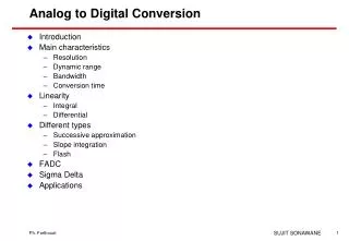
Analog to Digital Conversion. Introduction Main characteristics Resolution Dynamic range Bandwidth Conversion time Linearity Integral Differential Different types Successive approximation Slope integration Flash FADC Sigma Delta Applications. Analog to Digital Converter.

Analog to Digital Conversion
E N D
Presentation Transcript
Analog to Digital Conversion • Introduction • Main characteristics • Resolution • Dynamic range • Bandwidth • Conversion time • Linearity • Integral • Differential • Different types • Successive approximation • Slope integration • Flash • FADC • Sigma Delta • Applications SUJIT SONAWANE
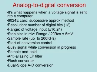
Analog to Digital Converter • Analog input - Digital output • Most of the time commercial ASICs • Converts voltage or current • What is to be converted? • Voltage, Current, Charge, Time • Analog input processing is necessary • To convert the measured quantity in a tension • To adapt the impedances • To filter • To adapt the amplitude • What is the expected resolution? • What is the dynamic range? • What is the expected linearity? • How often is a conversion needed? SUJIT SONAWANE
Resolution • An ADC is given as an n-bit ADC • The least significant bit gives the resolution of the ADC • Related to full scale if the ADC is linear • LSB = A/2n • Linear 8-bit ADC with a 1V full scale input • Resolution = 1/28 = 3.9 mV (0.39%) SUJIT SONAWANE
Dynamic range • Ratio between the minimum and the maximum amplitude to be measured • e.g. calorimeter signal 10 MeV to 2 TeV gives a 2 106 dynamic range • In case of linear system the dynamic range is related to the number of bits (and hence the resolution) • an 8-bit ADC has a 256 dynamic range • In case of large dynamic range (as for a calorimeter) some non-linearity has to be introduced • linear ADC for the previous example would require 21 bits! • Often used terms in physics: • n-bit resolution • n-bit dynamic range • example: • 8-bit resolution for a 12-bit dynamic range means that a signal in the range 1-4000 is measured with a resolution of 0.39% SUJIT SONAWANE
Conversion time and Bandwidth • How often can a conversion be done • a few ns to a few ms depending on the technology • 100 MHz FADC to slow sigma-delta • Input bandwidth • Maximum input signal bandwidth • Track and hold input circuitry • Conversion frequency (FADC) SUJIT SONAWANE
ADC transfer curve • Ideal ADC • Errors • Offset • Integral non-linearity • Differential non-linearity SUJIT SONAWANE
Non Linearity Integral linearity • Non linearity: maximum difference between the best linear fit and the ideal curve SUJIT SONAWANE
Differential non-linearity • Least Significant Bit (LSB) value should be constant but it is not • The difference with the ideal value shall not exceed 0.5 LSB • Easy way of seeing the effect • random input covering the full range • frequency histogram should be flat • differential non-linearity introduces structures SUJIT SONAWANE
Types of ADC • Successive approximation • Single slope integration • Dual slope integration • Flash ADC • Sigma-Delta SUJIT SONAWANE
Successive approximation • Compare the signal with an n-bit DAC output • Change the code until • DAC output = ADC input • An n-bit conversion requires n steps • Requires a Start and an End signals • Typical conversion time • 1 to 50 ms • Typical resolution • 8 to 12 bits • Cost • 15 to 600 CHF SUJIT SONAWANE
Vin - + Counting time StartConversion StartConversion Enable S Q R N-bit Output Counter C Clk Oscillator IN Single slope integration • Start to charge a capacitor at constant current • Count clock ticks during this time • Stop when the capacitor voltage reaches the input • Cannot reach high resolution • capacitor • comparator SUJIT SONAWANE
Charge with a currentproportional to the input Counting time Dual slope integration (Wilkinson) • Capacitor charged with a current proportional to the input during a fixed time • Discharge at constant current • Count of clock ticks during the discharge SUJIT SONAWANE
Dual slope integration (2) • Advantages • Capacitor value is not important although has to be of good quality • Comparator error can be canceled by beginning and ending each conversion cycle at the same voltage • Clock frequency errors can be cancelled by using the same clock to define the charge time • Typical resolution • 10 to 18 bit • Conversion time • Depends on the clock frequency SUJIT SONAWANE
Flash ADC • Direct measurement with 2n-1 comparators • Typical performance: • 4 to 10-12 bits • 15 to 300 MHz • High power • Half-Flash ADC • 2-step technique • 1st flash conversion with 1/2 the precision • Subtracted with a DAC • New flash conversion • Waveform digitizing applications SUJIT SONAWANE
X 4 - S&H 3-bit FADC 3-bit DAC 3-bit S&H Stage 1 Stage 2 Stage 3 Stage 4 4-bit FADC Input 3-bit 3-bit 3-bit 3-bit 4-bit Time Adjustment & Digital Error Correction 12-bit Flash ADC (cont) • Pipeline ADC • Input-to-output delay = n clocks for n stages • One output every clock cycle • Saves power (less comparators) SUJIT SONAWANE
q e(x) Effective number of bits • An n bit ADC introduces a quantization error • Effective number of bits of an n-bit FADC • n’ giving the correct SNR • Example: AD9235 12-bit 20 to 65 MHz • SNR = 70 dB • Effective number of bits = 11.4 • Encoding a signal (A/2) sinwt with A being the full scale will give an error • Signal to Noise Ratio SUJIT SONAWANE
Shannon Theorem • A signal x(t) has a spectral representation |X(f)|; X(f) = Fourier transform of x(t) • A signal x(t) after having been digitised at the frequency fs, has a spectral representation equal to the spectral representation of x(t) shifted every fs • If X(f) is not equal to zero when f > fs/2, there is spectrum overlapping • The Shannon theorem says that x(t) can be reconstructed after digitisation if the digitising frequency is at least twice the maximum frequency in x(t) spectral representation • This is mathematical only, as it supposes perfect filtering SUJIT SONAWANE
Example (1) • “Typical” physics pulse • 100 ns rising and falling edge • Effect of a digitisation at 10 MHz and 20 MHz SUJIT SONAWANE
Example (2) • 100 ns square pulse • Digitisation at 10 MHz and 20 MHz SUJIT SONAWANE
1/2*T0 +T0 -T0 Using FADC • Do not forget to make a frequency analysis of the signal • Any spectrum overlapping introduces noise • Take into account the effective number of bits • Filtering is necessary • Before digitisation (analog) to cut the input signal frequency spectrum • After digitisation (digital) to extract the signal frequency spectrum and to compensate the effect of digitisation over a finite time window SUJIT SONAWANE
|e(f)| q f e(x) -fs/2 +fs/2 Over-sampling ADC • If fs is higher than the frequency f0 of the signal to be measured then after filtering the error will become • Assuming the error is a white noise, its power spectral density is flat within the range [–fs/2,fs/2] SUJIT SONAWANE
Over-sampling ADC (cont) • The signal to noise ratio when encoding a signal (A/2) sinwt, with A being the full scale, will be • Hence it is possible to increase the resolution by increasing the sampling frequency and filtering • Example : an 8-bit ADC becomes a 9-bit ADC with an over-sampling factor of 4 • But the 8-bit ADC must meet the linearity requirement of a 9-bit SUJIT SONAWANE
- Input Output 1-bit ADC 1-bit DAC 1rst Order Sigma-Delta Modulator Sigma-Delta ADC • The output of this modulator is a digital stream • Average = Input • Over-sampling ratio M=fs/f0 SUJIT SONAWANE
Sigma-Delta ADC (cont) • The signal to noise ratio when encoding a signal (A/2) sinwt, with A being the full scale, will be • Gain of 1.5 bits per octave increase of M • M = 2350 to have a 16-bit ADC • Higher orders sigma-delta are implemented • Examples (Analog Devices) • 16-bit, 2.5 MHz • 24-bit, 1kHz The design of low-voltage, low-power sigma-delta modulators Shahriar Rabii & Bruce Wooley Kluwer academic publisher SUJIT SONAWANE
Resolution/Throughput Rate SUJIT SONAWANE
Power • Power is going down • Examples • 8-bit, 200MSPS: 1.3 mW/MSPS • 10-bit, 10 MSPS core used in ALICE TPC read-out: <20 mW • 24-bit, 1 kSPS: 45 mW SUJIT SONAWANE
Applications • In HEP we are facing large number of channels • The quantity to be measured depends on the type of detector • Charge in the case of a lead glass calorimeter with PM read-out • Voltage in the case of a lead glass calorimeter with triode and preamplifier shaper read-out • Low cost Charge integrating ADC for a LEP calorimeter • High speed peak sensing ADC for a neutrino experiment • Non linear ADC for an LHC experiment • FADC with numerical filtering for an LHC trigger application SUJIT SONAWANE
Charge integrating ADC (1) • High resolution: 12-bit • High dynamic range: 15-bit • High density: 96 channel per Fastbus board • Low speed: 1 ms conversion time • Low cost per channel • Principle: • Single ADC for 48 channels • Charge input integration and storage SUJIT SONAWANE
Charge integrating ADC (2) • Block diagram SUJIT SONAWANE
Charge integrating ADC (3) • Performance • 12-bit resolution, 15-bit dynamic range • Conversion time tcvt = 48 (tc + ts) = 960 µs • where tc = ADC conversion time = 12 µs • and ts = settling time for multiplexer and amplifiers = 8 µs. SUJIT SONAWANE
Peak sensing ADC (1) • 12-bit resolution • Low dead-time : 8 ms • Data buffering SUJIT SONAWANE
+ + - - C Peak sensing ADC (2) • Block diagram Vin FIFO ADC Read-out 12-bit Gate SUJIT SONAWANE
ADC for an LHC experiment (1) • ATLAS Liquid Argon calorimeter • High dynamic range: 16-bit • Shaping of the signal to minimise pile-up • Sampling every 25 ns (bunch crossing period) • Level-1 pipeline Shaping SUJIT SONAWANE
ADC for an LHC experiment (2) • Block diagram SUJIT SONAWANE
ADC for an LHC experiment (3) • Performance • Pedestal stability to 0.1 ADC counts • Noise equivalent to 20 MeV • Integral non-linearity below 0.25% • Conversion time : 25 ns per sample SUJIT SONAWANE
FADC for LHC trigger purpose (1) • Analog summation on the detector to form the trigger tower • Shaping time covers several bunch crossings • FADC and numerical filtering to: • Extract the energy • Extract the bunch crossing responsible for it SUJIT SONAWANE
FADC for LHC trigger purpose (2) • Block diagram SUJIT SONAWANE
FADC for LHC trigger purpose (3) • Filter algorithm : Finite Impulse Response SUJIT SONAWANE