CHAPTER 7: RELATIONS FOR 1D BEDLOAD TRANSPORT
390 likes | 592 Views
CHAPTER 7: RELATIONS FOR 1D BEDLOAD TRANSPORT. Let q b denote the volume bedload transport rate per unit width (sliding, rolling, saltating). It is reasonable to assume that q b increases with a measure of flow strength, such as depth-averaged flow velocity U or boundary shear stress b .

CHAPTER 7: RELATIONS FOR 1D BEDLOAD TRANSPORT
E N D
Presentation Transcript
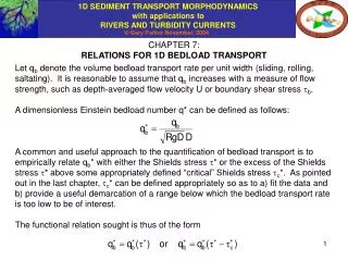
CHAPTER 7: RELATIONS FOR 1D BEDLOAD TRANSPORT Let qb denote the volume bedload transport rate per unit width (sliding, rolling, saltating). It is reasonable to assume that qb increases with a measure of flow strength, such as depth-averaged flow velocity U or boundary shear stress b. A dimensionless Einstein bedload number q* can be defined as follows: A common and useful approach to the quantification of bedload transport is to empirically relate qb* with either the Shields stress * or the excess of the Shields stress * above some appropriately defined “critical” Shields stress c*. As pointed out in the last chapter, c* can be defined appropriately so as to a) fit the data and b) provide a useful demarcation of a range below which the bedload transport rate is too low to be of interest. The functional relation sought is thus of the form
BEDLOAD TRANSPORT RELATION OF MEYER-PETER AND MÜLLER All the bedload relations in this chapter pertain to a flow condition known as “plane-bed” transport, i.e. transport in the absence of significant bedforms. The influence of bedforms on bedload transport rate will be considered in a later chapter. The “mother of all modern bedload transport relations” is that due to Meyer-Peter and Müller (1948) (MPM). It takes the form The relation was derived using flume data pertaining to well-sorted sediment in the gravel sizes. Recently Wong (2003) and Wong and Parker (submitted) found an error in the analysis of MPM. A re-analysis of the all the data pertaining to plane-bed transport used by MPM resulted in the corrected relation If the exponent of 1.5 is retained, the best-fit relation is
LIMITATIONS OF MPM The “critical Shields stress” c* of either 0.047 or 0.0495 in either the original or corrected MPM relation(s) must be considered as only a matter of convenience for correlating the data. This can be demonstrated as follows. Consider bankfull flow in a river. The bed shear stress at bankfull flow bbf can be estimated from the depth-slope product rule of normal flow: The corresponding Shields stress bf50* at bankfull flow is then estimated as where Ds50 denotes a surface median size. For the gravel-bed rivers presented in Chapter 3, however, the average value of bf50* was found to be about 0.05 (next page). According to MPM, then, these rivers can barely move sediment of the surface median size Ds50 at bankfull flow. Yet most such streams do move this size at bankfull flow, and often in significant quantities.
LIMITATIONS OF MPM contd. gravel-bed streams There is nothing intrinsically “wrong” with MPM. In a dimensionless sense, however, the flume data used to define it correspond to the very high end of the transport events that normally occur during floods in alluvial gravel-bed streams. While the relation is important in a historical sense, it is not the best relation to use with gravel-bed streams.
A SMORGASBORD OF BEDLOAD TRANSPORT RELATIONS FOR UNIFORM SEDIMENT Some commonly-quoted bedload transport relations with good data bases are given below. Einstein (1950) Ashida & Michiue (1972) Engelund & Fredsoe (1976) Fernandez Luque & van Beek (1976) Parker (1979) fit to Einstein (1950)
PLOTS OF BEDLOAD TRANSPORT RELATIONS E = Einstein AM = Ashida-Michiue EF = Engelund-Fredsoe P approx E = Parker approx of Einstein FLBSand = Fernandez Luque-van Beek, tc* = 0.038 FLBGrav = Fernandez Luque-van Beek, tc* = 0.0455
NOTES ON THE BEDLOAD TRANSPORT RELATIONS The bedload relation of Einstein (1950) contains no critical Shields number. This reflects his probabilistic philosophy. All of the relations except that of Einstein correspond to a relation of the form In the limit of high Shields number. In dimensioned form this becomes where K is a constant; for example in the case of Ashida-Michiue, K = 17. Note that in this limit the bedload transport rate becomes independent of grain size!! Some of the scatter between the relations is due to the face that c* should be a function of Rep. This is reflected in the discussion of the Fernandez Luque-van Beek relation in the next slide. (Recall that .) • Some of the scatter is also due to the fact that several of the relations have been plotted well outside of the data used to derive them. For example, in data used to derive Fernandez Luque-van Beek, * never exceeded 0.11, whereas the plot extends to * = 1.
NOTES ON THE RELATION OF FERNANDEZ LUQUE AND VAN BEEK In the experiments on which the relation is based; a) Streamwise bed slope angle varied from near 0 to 22. The material tested included five grain sizes and three specific gravities, as given below; also listed are the values of Rep and the critical Shields number co* determined empirically at near vanishing bed slope angle. c) It is thus possible to check the effect of Rep and on the transport relation of Fernandez Luque and van Beek (FLvB).
CRITICAL SHIELDS NUMBER IN THE RELATION OF FLvB The experimental values of co* generally track the modified Shields relation of Chapter 6, but are high by a factor ~ 2. This reflects the fact that they correspond to a condition of “very small” transport determined in a consistent way (see original reference). .
CRITICAL SHIELDS NUMBER IN THE RELATION OF FLvB contd. The ratio c*/co* decreases with streamwise angle as predicted by the relation of Chapter 6, but to obtain good agreement r must be set to the rather high value of 47 (c = 1.07). .
SHEET FLOW • For values of * < a threshold value sheet*, bedload is localized in terms of rolling, sliding and saltating grains that exchange only with the immediate bed surface. • When s* > sheet* the bedload layer devolves into a sliding layer of grains that can be several grains thick. Sheet flows occur in unidirectional river flows as well as bidirectional flows in the surf zone. • Values of sheet* have been variously estimated as 0.5 ~ 1.5. (Horikawa, 1988, Fredsoe and Diegaard, 1994, Dohmen-Jannsen, 1999; Gao, 2003). The parameter sheet* appears to decrease with increasing Froude number. • Wilson (1966) has estimated the bedload transport rate in the sheet flow regime as obeying a relation of the form • All the previously presented bedload relations except that of Einstein also devolve to a relation of the above form for large *, with K varying between 3.97 and 18.74.
A VIEW OF SHEET FLOW TRANSPORT Double-click on the image to run the video. D = 0.116 mm S = 0.035 U = 1.05 m/s Fr = 1.85 sheet* = 0.51 rte-booksheetpeng.mpg: to run without relinking, download to same folder as PowerPoint presentations. Video clip courtesy P. Gao and A. Abrahams; Gao (2003)
MECHANISTIC DERIVATIONS OF BEDLOAD TRANSPORT RELATIONS A number of mechanistic derivations of bedload transport relations are available. These are basically of two types, based on two forms for bedload continuity. Let bl = the volume of sediment in bedload transport per unit area, ubl = the mean velocity of bedload particles, Ebl = the volume rate of entrainment of bed particles into bedload movement (rolling, sliding or saltation, not suspension) and Lsbl = the average step length of a bedload particle (from entrainment to deposition, usually including many saltations). The following continuity relations then hold: In a Bagnoldean approach, separate predictors are developed for ubl and bl, the latter determined from the Bagnold constraint (Bagnold, 1956). Models of this type include the macroscopic models of Ashida and Michiue (1972) and Engelund and Fredsoe (1976), and the saltation models of Wiberg and Smith (1985, 1989), Sekine and Kikkawa (1992), and Nino and Garcia (1994a,b). Recently, however, Seminara et al. (2003) have shown that the Bagnold constraint is not generally correct. In the Einsteinean approach the goal is to develop predictors for Ebl and Lsbl. It is the former relation that is particularly difficult to achieve. Models of this type include the Einstein (1950), Tsujimoto (e.g. 1991) and Parker et al. (2003).
CALCULATIONS WITH BEDLOAD TRANSPORT RELATIONS • To perform calculations with any of the previous bedload transport relations, it is necessary to specify: • the submerged specific gravity R of the sediment; • a representative grain size exposed on the bed surface, e.g. surface geometric mean size Dsg or surface median size Ds50, to be used as the characteristic size D in the relation; • and a value for the shear velocity of the flow u* (and thus b). • Once these parameters are specified, * = (u*)2/(RgD) is computed, qb* is calculated from the bedload transport relation, and the volume bedload transport rate per unit width is computed as qb = (RgD)1/2Dqb*. • The shear velocity u* is computed from the flow field using the techniques of Chapter 5. For example, in the case of normal flow satisfying the Manning-Strickler resistance relation,
ALTERNATIVE DIMENSIONLESS BEDLOAD TRANSPORT Again, the case under consideration is plane-bed bedload transport (no bedforms). As a preliminary, define a dimensionless sediment transport rate W* as Now all previously presented bedload transport rates for uniform sediment can be rewritten in terms of W* as a function of *: Einstein (1950) Ashida & Michiue (1972) Engelund & Fredsoe (1976) Fernandez Luque & van Beek (1976) Parker (1979) fit to Einstein (1950)
SURFACE-BASED BEDLOAD TRANSPORT FORMULATION FOR MIXTURES Consider the bedload transport of a mixture of sizes. The thickness La of the active (surface) layer of the bed with which bedload particles exchange is given by as where Ds90 is the size in the surface (active) layer such that 90 percent of the material is finer, and na is an order-one dimensionless constant (in the range 1 ~ 2). Divide the bed material into N grain size ranges, each with characteristic size Di, and let Fi denote the fraction of material in the surface (active) layer in the ith size range. The volume bedload transport rate per unit width of sediment in the ith grain size range is denoted as qbi. The total volume bedload transport rate per unit width is denoted as qbT, and the fraction of bedload in the ith grain size range is pbi, where Now in analogy to *, q* and W*, define the dimensionless grain size specific Shields number i*, grain size specific Einstein number qi* and dimensionless grain size specific bedload transport rate Wi* as
SURFACE-BASED BEDLOAD TRANSPORT FORMULATION contd. It is now assumed that a functional relation exists between qi* (Wi*) and i*, so that The bedload transport rate of sediment in the ith grain size range is thus given as According to this formulation, if the grain size range is not represented in the surface (active) layer, it will not be represented in the bedload transport.
BEDLOAD RELATION FOR MIXTURES DUE TO ASHIDA AND MICHIUE (1972) Basic transport relation Effective critical Shields stress for surface geometric mean size Note This relation has been modified slightly from the original formulation. Here the relation specifically uses surface fractions Fi, and surface geometric mean size Dsg is specified in preference to the original arithmetic mean size Dsm = DiFi. Modified version of Egiazaroff (1965) hiding function
BEDLOAD RELATION FOR MIXTURES DUE TO PARKER (1990a,b) This relation is appropriate only for the computation of gravel bedload transport rates in gravel-bed streams. In computing Wi*, Fi must be renormalized so that the sand is removed, and the remaining gravel fractions sum to unity, Fi = 1. The method is based on surface geometric size Dsg and surface arithmetic standard deviation s on the scale, both computed from the renormalized fractions Fi. In the above O and O are set functions of sgospecified in the next slide.
BEDLOAD RELATION FOR MIXTURES DUE TO PARKER (1990a,b) contd. o o It is not necessary to use the above chart. The calculations can be performed using the Visual Basic programs in RTe-bookAcronym1.xls
BEDLOAD RELATION FOR MIXTURES DUE TO PARKER (1990a,b) contd. An example of the renormalization to remove sand is given below.
PROGRAMMING IN VISUAL BASIC FOR APPLICATIONS The Microsoft Excel workbook RTe-bookAcronym1.xls is an example of a workbook in this e-book that uses code written in Visual Basic for Applications (VBA). VBA is built directly into Excel, so that anyone who has Excel (versions 2000 or later) can execute the code directly from the relevant worksheet in the workbook RTe-bookAcronym1.xls. The relevant code is contained in three modules, Module1, Module2 and Module3 of the workbook, which may be accessed from the Visual Basic Editor. All the code in this e-book is written in VBA in Excel modules. A self-teaching tutorial in VBA is contained in the workbook RTe-bookIntroVBA.xls. Going though the tutorial will not only help the reader understand the material in this e-book, but also allow the reader to write, execute and distribute similar code. To take the tutorial, open RTe-bookIntroVBA.xls and follow the instructions.
NOTES ON Rte-bookAcronym1.xls The workbook RTe-bookAcronym1.xls provides interfaces for three different implementations. In the implementation of “Acronym1” the user inputs the specific gravity of the sediment R+1, the shear velocity of the flow and the grain size distribution of the bed material. The code computes the magnitude and size distribution of the bedload transport. In the implementation of “Acronym1_R” the user inputs the specific gravity of the sediment R+1, the flow discharge Q, the bed slope S, the channel width B, the parameter nk relating the roughness height ks to the surface size Ds90 and the grain size distribution of the bed material. The code computes the shear velocity using a Manning-Strickler resistance formulation and the assumption of normal flow, and then computes the magnitude and size distribution of the bedload transport. The implementation of “Acronym1_D” uses the same formulation as “Acronym1_R”, but allows specification of a flow duration curve so that average annual gravel transport rate and grain size distribution can be computed.
EXAMPLE: INTERFACE FOR “Acronym1” IN Rte-bookAcronym1.xls
BEDLOAD RELATION FOR MIXTURES DUE TO WILCOCK AND CROWE (2003) The sand is not excluded in the fractions Fi used to compute Wi*. The method is based on the surface geometric mean size Dsg and fraction sand in the surface layer Fs.
EFFECT OF SAND CONTENT IN THE SURFACE LAYER ON GRAVEL MOBILITY IN A GRAVEL-BED STREAM Wilcock and Crowe (2003) have shown that increasing sand content in the bed surface layer of a gravel-bed stream renders the surface gravel more mobile. This effect is captured in their relationship between the reference Shields number for the surface geometric mean size (a surrogate for a critical Shields number) and the fraction sand Fs in the surface layer: Note how decreases as Fs increases. The surface layers of gravel-bed streams rarely contain more than 30% sand; beyond this point the gravel tends to be buried under pure sand.
BEDLOAD RELATION FOR MIXTURES DUE TO POWELL, REID AND LARONNE (2001) The sand is excluded in the fractions Fi used to compute Wi*. The method is based on the surface median size Ds50, computed after excluding sand.. More information about bedload transport relations for mixtures can be found in Parker (in press; downloadable from http://www.ce.umn.edu/~parker/).
SAMPLE CALCULATIONS OF BEDLOAD TRANSPORT RATE OF MIXTURES Assumed grain size distribution of the bed surface: Dsg = surface geometric mean, sg = surface geometric standard deviation, Fs = fraction sand in surface layer. Dsg = 40.7 mm, sg = 2.36 (sand excluded) Dsg = 22.3 mm, sg = 4.93, Fs = 0.16
SAMPLE CALCULATIONS, MIXTURES contd. Other input parameters: R = 1.65 u* = 0.15 to 0.40 m/s Relations used: A-M = Ashida and Michiue (1972), sand not excluded P = Parker (1990), sand excluded P-R-L = Powell et al. (2001), sand excluded W-C = Wilcock and Crowe (2003), sand not excluded Output parameters qG = volume gravel bedload transport rate per unit width DGg = geometric mean size of the gravel portion of the transport Gg = geometric standard deviation of the gravel portion of the bedload pG = fraction gravel in the bedload transport (only for A-M and W-C): fraction sand = 1 - pG
COMPUTATIONS OF ANNUAL BEDLOAD YIELD It is necessary to have a flow duration curve to perform the calculation. The flow duration curve specifies the fraction of time a given water discharge is exceeded, as a function of water discharge. This curve is divided into M bins k = 1 to M, such that pQk specifies the fraction of time the flow is in range k with characteristic discharge Qk. The value u*k must be computed for each range. For example, in the case of normal flow with constant width B, the Manning-Strickler resistance relation from Chapter 5 yields The grain size distribution of the bed material must be specified; ks can be computed as 2 Ds90 (for a plane bed). Once u*,k is computed, either qb,k (material approximated as uniform) or qbi,k (mixtures) is computed for each flow range, and the annual sediment yield qba or total yield qbTa and grain size fractions of the yield pai are given as Expect the flood flows to contribute disproportionately to the annual sediment yield. An implementation is given in “Acronym1_D” of Rte-bookAcronym1.xls .
REFERENCES FOR CHAPTER 7 Ashida, K. and M. Michiue, 1972, Study on hydraulic resistance and bedload transport rate in alluvial streams, Transactions, Japan Society of Civil Engineering, 206: 59-69 (in Japanese). Bagnold, R. A., 1956, The flow of cohesionless grains in fluids, Philos Trans. R. Soc. LondonA, 249, 235-297. Dohmen-Janssen, M., 1999, Grain size influence on sediment transport in oscillatory sheet flow, Ph.D. thesis, Technical University of Delft, the Netherlands, 246 p. Einstein, H. A., 1950, The Bed-load Function for Sediment Transportation in Open Channel Flows, Technical Bulletin 1026, U.S. Dept. of the Army, Soil Conservation Service. Egiazaroff, I. V., 1965, Calculation of nonuniform sediment concentrations, Journal of Hydraulic Engineering, 91(4), 225-247. Engelund, F. and J. Fredsoe, 1976, A sediment transport model for straight alluvial channels, Nordic Hydrology, 7, 293-306. Fernandez Luque, R. and R. van Beek, 1976, Erosion and transport of bedload sediment, Journal of Hydraulic Research, 14(2): 127-144. Fredsoe, J. and Deigaard, R., 1994, Mechanics of Coastal Sediment Transport, World Scientific, ISBN 9810208405, 369 p. Gao, P., 2003, Mechanics of bedload transport in the saltation and sheetflow regimes, Ph.D. thesis, Department of Geography, University of Buffalo, State University of New York Horikawa, K., 1988, Nearshore Dynamics and Coastal Processes, University of Tokyo Press, 522 p.
REFERENCES FOR CHAPTER 7 contd. Meyer-Peter, E. and Müller, R., 1948, Formulas for Bed-Load Transport, Proceedings, 2nd Congress, International Association of Hydraulic Research, Stockholm: 39-64. Nino, Y. and Garcia, M., 1994a, Gravel saltation, 1, Experiments, Water Resour. Res., 30(6), 1907-1914. Nino, Y. and Garcia, M., 1994b, Gravel saltation, 2, Modelling, Water Resour. Res., 30(6), 1915- 1924. Parker, G., 1979, Hydraulic geometry of active gravel rivers, Journal of Hydraulic Engineering, 105(9), 1185‑1201. Parker, G., 1990a, Surface-based bedload transport relation for gravel rivers, Journal of Hydraulic Research, 28(4): 417-436. Parker, G., 1990b, The ACRONYM Series of PASCAL Programs for Computing Bedload Transport in Gravel Rivers, External Memorandum M-200, St. Anthony Falls Laboratory, University of Minnesota, Minneapolis, Minnesota USA. Parker, G., Solari, L. and Seminara, G., 2003, Bedload at low Shields stress on arbitrarily sloping beds: alternative entrainment formulation, Water Resources Research, 39(7), 1183, doi:10.1029/2001WR001253, 2003. Parker, G., in press, Transport of gravel and sediment mixtures, ASCE Manual 54, Sediment Engineering, ASCE, Chapter 3, downloadable at http://cee.uiuc.edu/people/parkerg/manual_54.htm . Powell, D. M., Reid, I. and Laronne, J. B., 2001, Evolution of bedload grain-size distribution with increasing flow strength and the effect of flow duration on the caliber of bedload sediment yield in ephemeral gravel-bed rivers, Water Resources Research, 37(5), 1463-1474.
REFERENCES FOR CHAPTER 7 contd. Sekine, M. and Kikkawa, H., 1992, Mechanics of saltating grains, J. Hydraul. Eng., 118(4), 536-558. Seminara, G., Solari, L. and Parker, G., 2002, Bedload at low Shields stress on arbitrarily sloping beds: failure of the Bagnold hypothesis, Water Resources Research, 38(11), 1249, doi:10.1029/2001WR000681. Tsujimoto, T., 1991, Mechanics of Sediment Transport of Graded Materials and Fluvial Sorting, Report, Faculty of Engineering, Kanazawa University, Japan (in Japanese and English). Wiberg, P. L. and Smith, J. D., 1985, A theoretical model for saltating grains in water, J. Geophys. Res., 90(C4), 7341-7354. Wiberg, P. L. and Smith, J. D., 1989, Model for calculating bedload transport of sediment, J. Hydraul. Eng, 115(1), 101-123. Wilcock, P. R., and Crowe, J. C., 2003, Surface-based transport model for mixed-size sediment, Journal of Hydraulic Engineering, 129(2), 120-128. Wilson, K. C., 1966, Bed load transport at high shear stresses, Journal of Hydraulic Engineering, 92(6), 49-59. Wong, M., 2003, Does the bedload equation of Meyer-Peter and Müller fit its own data?, Proceedings, 30th Congress, International Association of Hydraulic Research, Thessaloniki, J.F.K. Competition Volume: 73-80. Wong, M. and Parker, G., submitted, The bedload transport relation of Meyer-Peter and Müller overpredicts by a factor of two, Journal of Hydraulic Engineering, downloadable at http://cee.uiuc.edu/people/parkerg/preprints.htm .