Download
1 / 32
350 likes | 584 Views
Simulink. Simulink is a graphical extension to MATLAB for modeling and simulation of systems. In Simulink, systems are drawn on screen as block diagrams. Many elements of block diagrams are available such as oscilloscopes. Getting started.

E N D
Simulink Simulink is a graphical extension to MATLAB for modeling and simulation of systems. In Simulink, systems are drawn on screen as block diagrams. Many elements of block diagrams are available such as oscilloscopes
Getting started • Simulink is started from the MATLAB command prompt by entering the following command: • >>simulink • Alternatively, you can hit the New Simulink Model button at the top of the MATLAB command window
When it starts, Simulink brings up two windows. The first is the main Simulink window, which appears as:
The second window is a blank, untitled, model window. This is the window into which a new model can be drawn.
Model Files • In Simulink, a model is a collection of blocks which, in general, represents a system. • A new model can be created by selecting New from the File menu in any Simulink window (or by hitting Ctrl+N). • In addition, to drawing a model into a blank model window, previously saved model files can be loaded either from the File menu or from the MATLAB command prompt.
Save your model • You might create a new folder, like the one shown below, called simulink_files • Use the .mdl suffix when saving
Basic Elements • There are two major classes of items in Simulink: blocks and lines. • Blocks are used to generate, modify, combine, output, and display signals. • Lines are used to transfer signals from one block to another.
Blocks • There are several general classes of blocks: • Sources: Used to generate various signals • Sinks: Used to output or display signals • Discrete: Linear, discrete-time system elements (transfer functions, state-space models, etc.) • Linear: Linear, continuous-time system elements and connections (summing junctions, gains, etc.) • Nonlinear: Nonlinear operators (arbitrary functions, saturation, delay, etc.) • Connections: Multiplex, Demultiplex, System Macros, etc.
Blocks have zero to several input terminals and zero to several output terminals. • Unused input terminals are indicated by a small open triangle. • Unused output terminals are indicated by a small triangular point. • The block shown below has an unused input terminal on the left and an unused output terminal on the right.
Lines • Lines transmit signals in the direction indicated by the arrow. • Lines must always transmit signals from the output terminal of one block to the input terminal of another block. • On exception to this is a line can tap off of another line, splitting the signal to each of two destination blocks, as shown in next+ slide
Lines can never inject a signal into another line; lines must be combined through the use of a block such as a summing junction.
Simple Example • The simple model consists of three blocks: Step, Transfer Fcn, and Scope. • The Step is a source block from which a step input signal originates. • This signal is transferred through the line in the direction indicated by the arrow to the Transfer Function linear block. • The Transfer Function modifies its input signal and outputs a new signal on a line to the Scope. • The Scope is a sink block used to display a signal much like an oscilloscope.
Modifying Blocks A block can be modified by double-clicking on it. For example, if you double-click on the "Transfer Fcn" block in the simple model, you will see the following dialog box.
This dialog box contains fields for the numerator and the denominator of the block's transfer function. • By entering a vector containing the coefficients of the desired numerator or denominator polynomial, the desired transfer function can be entered. For example, to change the denominator to s^2+2s+1, enter the following into the denominator field: [1 2 1] and hit the close button, the model window will change to the following,
which reflects the change in the denominator of the transfer function.
The "step" block can also be double-clicked, bringing up the following dialog box.
The default parameters in this dialog box generate a step function occurring at time=1 sec, from an initial level of zero to a level of 1. (in other words, a unit step at t=1). • Each of these parameters can be changed. Close this dialog before continuing. • One more block is the "Scope" block. Double clicking on this brings up a blank oscilloscope screen.
When a simulation is performed, the signal which feeds into the scope will be displayed in this window.
Running Simulations To run a simulation, we will work with the following model file: simple2.mdl
Before running a simulation of this system, first open the scope window by double-clicking on the scope block. • Then, to start the simulation, either select Start from the Simulation menu (as shown below) or hit Ctrl-T in the model window.
The simulation should run very quickly and the scope window will appear as shown below. • Note that the simulation output (shown in yellow) is at a very low level relative to the axes of the scope. • To fix this, hit the autoscale button (binoculars), which will rescale the axes as shown below
Note that the step response does not begin until t=1. This can be changed by double-clicking on the "step" block. • Now, we will change the parameters of the system and simulate the system again. • Double-click on the "Transfer Fcn" block in the model window and change the denominator to • [1 20 400]
Re-run the simulation (hit Ctrl-T) and you should see what appears as a flat line in the scope window. • Hit the autoscale button, and you should see the following in the scope window. • Notice that the autoscale button only changes the vertical axis.
In the model window, select Parameters from the Simulation menu. You will see the following dialog box.
There are many simulation parameter options; we will only be concerned with the start and stop times, which tell Simulink over what time period to perform the simulation. • Change Start time from 0.0 to 0.8 (since the step doesn't occur until t=1.0. • Change Stop time from 10.0 to 2.0, which should be only shortly after the system settles. • Close the dialog box and rerun the simulation. • After hitting the autoscale button, the scope window should provide a much better display of the step response as shown below.
Block Libraries • Simulink contains a large number of blocks from which models can be build. • These blocks are arranged in Block Libraries which are accessed in the main Simulink window shown below
Each icon in the main Simulink window can be double clicked to bring up the corresponding block library. • Blocks in each library can then be dragged into a model window to build a model.
Assignment #1 List down all blocks in these libraries • Sources • Sinks • Discrete • Linear • Nonlinear • Connections
Assignment#1 Draw the given model, save it as model.mdl Run it and show simulation result Also write all steps for drawing and running the “model.mdl”