Root Locus Analysis (1)
Root Locus Analysis (1). Hany Ferdinando Dept. of Electrical Eng. Petra Christian University. General Overview. This section discusses how to plot the Root Locus method Step by step procedure is used inline with an example Finally, some comments are given as the complement for this section.


Root Locus Analysis (1)
E N D
Presentation Transcript
Root Locus Analysis (1) Hany Ferdinando Dept. of Electrical Eng. Petra Christian University
General Overview • This section discusses how to plot the Root Locus method • Step by step procedure is used inline with an example • Finally, some comments are given as the complement for this section
Why Root Locus • Closed-loop poles’ location determine the stability of the system • Closed-loop poles’ location is influenced as the gain is varied • Root locus plot gives designer information how the gain variation influences the stability of the system
Important Notes: • Poles are drawn as ‘x’ while zeros are drawn as ‘o’ • Gain at poles is zero, while gain at zeros is infinity • Pole is the starting point and it must finish at zero; therefore, for every pole there should be corresponding zero • Root locus is plot on the s plane
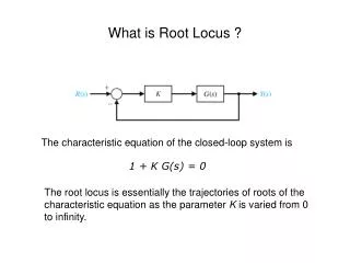
R(s) C(s) G(s) + - H(s) Standardization 1 + G(s)H(s) = 0 Find Characteristic Equation!!
How to make it? • Start from the characteristic equation • Locate the poles and zeros on the s plane • Determine the root loci on the real axis • Determine the asymptotes of the root loci • Find the breakaway and break-in points • Determines the angle of departure (angle of arrival) from complex poles (zeros) • Find the points where the root loci may cross the imaginary axis
Example (1) 1. Start from the characteristic equation
Example (2) 2. Locate the poles and zeros on the s plane
Example (3) 3. Determine the root loci on the real axis
Example (4a) 4. Determine the asymptotes of the root loci
Example (4b) 4. Determine the asymptotes of the root loci
Example (5) From the characteristic equation, find then calculate… s = -0.4266 and s = -1.5744 5. Find the breakaway and break-in point
Example (6) This example has no complex poles and zeros, therefore, this step can be skipped!!! qpole= 0 – sum from pole + sum from zero qzero = 0 – sum from zero + sum from pole 6. Determine the angle from complex pole/zero
Example (7) Do this part by substituting jw for all s in the characteristic equation w = ±√2, K = 6 or w = 0, K = 0 7. Find the points where the root loci may cross the imaginary axis
Comments • nth degree algebraic equation in s • If n-m≥2 then a1 is negative sum of the roots of the equation and is independent of K • It means if some roots move on the locus toward the left as K increased then the other roots must move towards the right as K is increased
Root Locus in Matlab Function rlocus(num,den) draws the Root Locus of a system. Another version in state space is rlocus(A,B,C,D) The characteristic equation Those functions are for negative feedback (normal transfer function)
Next… Topic for the next meeting is Root Locus in positive feedback