Root Locus Plotting Rules and Conditions | November 8, 2012
Understand key conditions for plotting the root locus of an open-loop transfer function, including magnitude and argument conditions, symmetry rules, asymptotes, breakaway and break-in points, and gain considerations. Learn about the characteristics of the root locus and apply rules to draw it effectively.


Root Locus Plotting Rules and Conditions | November 8, 2012
E N D
Presentation Transcript
Chapter 5: Root Locus Nov. 8, 2012
Key conditions for Plotting Root Locus Given open-loop transfer function Gk(s) Characteristic equation Magnitude Condition and Argument Condition
5-3 Rules for Plotting Root Locus 5.3.1 Rules Rule 1: Starting and end points end starting 1)For Kg=0, we can get from magnitude equation that 2) For Kg→+∞, it may result in one of the following facts Using Magnitude Equation s→+∞ (n>m) Rule #1: The locus starts at a pole for Kg=0 and finishes at a zero or infinity when Kg=+∞.
Poles and zeros at infinity Gk(s) has a zero at infinity if Gk (s→+∞) →0 Gk(s) has a pole at infinity if Gk (s→+∞) → +∞ Example This open-loop transfer function has three poles, 0,-1,-2. It has no finite zeros. For large s, we can see that . So this open-loop transfer function has three (n-m) zeros at infinity.
Rule #2: The number of segments equals to the number of poles of open-loop transfer function. m segments end at the zeros, and (n-m) segments goes to infinity. Rule 2: Number of segments Sometimes, max{m,n} Rule 3: Symmetry rule Rule #3: The loci are symmetrical about the real axis since complex roots are always in conjugate pairs.
S1 Rule 4: Segments of the real axis Segments of the real axis to the left of an odd number of poles and zeros are segments of the root locus, remembering that complex poles or zeros have no effect. Using Argument Equation
s s Example Argument equation For complex zeros and poles For real zeros and poles on the right Real-axis segments are to the left of an odd number of real-axis finite poles/zeros.
60o 5. Asymptotes of locus as s Approaches infinity The asymptotes intersect the real axis at σ, where The intercept σ can be obtained by applying the theory of equations. The angle between asymptote and positive real axis is To obey the symmetry rules, the negative real axis is one asymptote when n-m is odd. Using Argument Equation
Example This open-loop transfer function has three finite poles and three zeros at infinity. (n-m) segments go to zeros at infinity. Assume the root of closed-loop system s1 at infinity has the same angle to each finite zero or pole.
Break-in point Breakaway point Rule 6: Breakaway and Break-in Points on the Real Axis When the root locus has segments on the real axis between two poles, there must be a point at which the two segments break away from the real axis and enter the complex region. For two finite zeros or one finite zero and one at infinity, the segments are coming from complex region and enter the real axis. Using Magnitude Equation
Breakaway point Kg starts with zero at the poles. There is a point somewhere the Kg for the two segments simultaneously reach a maximum value. Break-in point The break-in point is that the value of Kg is a minimum between two zeros. • Express Kgas a function of s • Differentiating the function with respect to s equals to zero and solve for s How?
Characteristic equation Assuming there are r repeated roots at the point S1, F(s)can be rewritten into With the solution of s, we can get Kg. For positive Kg, the corresponding point may be the breakaway or break-in point. Use the following necessary condition
Example Alternatively, we can solve for real s.
j3.74 Example : -j3.74 Substitute s=jw =0 =0 Rule #7: The point may be obtained by substituting s=jωinto the characteristic equation and solving for ω. Rule 7: The point where the locus crosses the imaginary axis Characteristic equation s=±j3.74
Characteristic equation: Routh array (2) Utilize Routh’s Stability Criterion 1 14 5 10+k =0 10+k k = 60
8. The angles of emergence and entry The angle of emergence from complex poles is given by Angles of the vectors from all other open-loop poles to the pole in question Angles of the vectors from the open-loop zeros to the complex pole in question
The angle of entry into a complex zero is given by Angles of the vectors from all other open-loop zeros to the zero in question Angles of the vectors from the open-loop poles to the complex zero in question
135o 33.5o 63.5o 90o Example: Given the open-loop transfer function draw the angle of emergence from complex poles.
Rule 9: The gain at a selected point st on the locus is obtained by applying Magnitude Equation To locate a point with specified gain, use trial and error. Moving st toward the poles reduces the gain. Moving st away from the poles increases the gain. Rule 10: The sum of real parts of the closed-loop poles is constant, independent of Kg, and equal to the sum of the real parts of the open-loop poles.
=5.818 =0.172 -3 -2 -1 Example 5.2.1: Given the open-loop transfer function, please draw the root locus. 6.Breakaway and break-in points 1.Draw the open-loop poles and zeros 2. Two segments 4. Segments on real axis 3.Symmetry 5.Asymptote zero pole pole breakaway Break-in
Example 5.2.2: j3.16 =121 =121 -j3.16 484-4 =0 get =121 • Find poles and zeros 7.The point where the locus across the imaginary axis 6. Breakaway and break-in points 3. Symmetry 5. Asymptote 2. 4 segments 4. No segments on real axis Breakaway -1 2020/1/5 23
-2 -1 5.Points across the imaginary axis 4. Breakaway and break-in points 2. Segments on real axis 3. Asymptotes • Open-loop poles and zeros Example 5.2.3 j1.414 K=6 -0.42 =0 K=6 -j1.414 K=6
Example 5.2.4 j s1 0 s2