Download
1 / 57
590 likes | 817 Views
Chapter 6 Root-Locus Analysis. 6.1 Introduction.

E N D
Chapter 6 Root-Locus Analysis 6.1 Introduction - In some systems simple gain adjustment may move the closed-loop poles to desired locations. Then the design problem may become the selection of an appropriate gain value. If the gain adjustment alone does not yield a desired result, addition of a compensator to the system will become necessary.
Unless otherwise stated, we shall assume that the gain of the open-loop transfer function is the parameter to be varied through all values, from zero to infinity. - By using the root-locus method the designer can predict the effects on the location of the closed-loop poles of varying the gain value or adding open-loop poles and/or open-loop zeros.
- The values of s that fulfill both the angle and magnitude conditions are the roots of the characteristic equation, or the closed-loop poles. • A locus of the points in the complex plane satisfying the angle condition alone is the root locus. - The roots of the characteristic equation (the closed-loop poles) corresponding to a given value of the gain can be determined from the magnitude condition.
- Begin sketching the root loci of a system by the root-locus method.For example, if G(s)H (s) is given by
Figure 6-2 (a) and (b) Diagrams showing angle measurements from open-loop poles and open-loop zero to test point s.
- The number of individual root loci for this system is three, which is the same as the number of open-loop poles.
- If a root locus lies between two adjacent open-loop poles on the real axis, then there exists at least one breakaway point between the two poles. - If the root locus lies between two adjacent zeros (one zero may be located at -) on the real axis, then there always exists at least one break-in point between the two zeros. -If the root locus lies between an open-loop pole and a zero (finite or infinite) on the real axis, then there may exist no breakaway or break-in points or there may exist both breakaway and break-in points.
- The angle of departure (or angle of arrival) of the root locus from a complex pole (or at a complex zero) can be found by subtracting from 180 the sum of all the angles of vectors from all other poles and zeros to the complex pole (or complex zero) in question, with appropriate signs included.
Figure 6-12 Construction of the root locus. [Angle of departure =180°- (ϴ1+ϴ2 )+Φ.]
Figure 6-20 Root-locus plot of system defined in state space, where A, B, C, and D are as given by Equation (6–15).