Download
1 / 52
520 likes | 603 Views
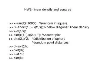
HW2- linear density and squares. >> x=rand(2,10000); %uniform in square >> ix=find(x(1,:)<x(2,:));% below diagonal: linear density >> x=x(:,ix); >> plot(x(1,:),x(2,:),'*'); %scatter plot >> d=x(2,:)*2; %distribution of sphere %random point distances

E N D
HW2- linear density and squares >> x=rand(2,10000); %uniform in square >> ix=find(x(1,:)<x(2,:));% below diagonal: linear density >> x=x(:,ix); >> plot(x(1,:),x(2,:),'*'); %scatter plot >> d=x(2,:)*2; %distribution of sphere %random point distances >> d=sort(d); >> plot(d); >> k=d.^2; >> plot(k);
>> mean (d) ans =1.3384 >> median(d) ans =1.4239 >> mean(k) ans =2.0085 >> median(k) ans =2.0275
Rejection sampling: Y-coordinates have linear density function
Plot of cdf of d Plot of cdf of d^2
Non-informative, proper and improper priors • For real quantity bounded to interval,standard prior is uniform distribution • For real quantity, unbounded, standard is uniform - but with what density? • For real quantity on half-open interval, standard prior is f(s)=1/s - but integral diverges! • Divergent priors are called improper -they can only be used with convergent likelihoods
Occurence table probability Uniform prior:
Non-parametric inference • How to perform inference about a distribution without assuming a distribution family? • A distribution over reals can be approximated by a piecewise uniform distribution a mixture of real distributions • But how many parts? This is non-parametric inference
Non-parametric inferenceChange-points, Rao-Blackwell • Given times for events (eg coal-mining disasters)Infer a piecewise constant intensity function(change-point problem) • State is set of change-points with intensities inbetween • But how many pieces? This is non-parametric inference • MCMC: Given current state, propose change in segment bounadry or intensity • But it is possible to integrate out intensities proposed
Probability ratio in MCMC For a proposed merge of intervals j and j+1, with sizesproportional to (,1-), were the counts and obtained by tossing a ‘coin’ with success probability or not? Compute model probability ratio as in HW1. Also, the total number of breakpoints has prior distribution Poisson with parameter (average) . Probability ratio in favor of split :
Mixture of Normalselimination of nuisance parameters (integrate using normalization constant of Gaussian and Gamma distributions)
Matlab Mixture of Normals, MCMC (AutoClass method) function [lh,lab,trlpost,trm,trstd,trlab,trct,nbounc]= mmnonu1(x,N,k,labi,NN); %[lh,lab,trlpost,trm,trstd,trlab,trct,nbounc]= % MMNONU1(x,N,k,labi,NN); %inputs % 1D MCMC mixture modelling, % x - 1D data column vector % N - MCMC iterations. % k - number of components %lab,labi - component labelling of data vector) % NN - thinning (optional)
Matlab Mixture of Normals, MCMC function [lab,trlh,trm,trstd,trlab,trct,nbounc]= mmnonu1(x,N,k,labi,NN); %[lh,lab,trlpost,trm,trstd,trlab,trct,nbounc]= % MMNONU1(x,N,k,labi,NN); %outputs %trlh - thinned trace of log probability (optional) %trm - thinned trace of means vector (optional) %trstd - thinned vector of standard deviations (optional) %trlab - thinned trace of labels vector (size(x,1) by N/NN (optional) %trct - thinned trace of mixing proportions
Matlab Mixture of Normals, MCMC N=10000; NN=100; x=[randn(100,1)-1;randn(100,1)*3;randn(100,1)+1]; % 3 components synthetic data k=2; labi=ceil(rand(size(x))*2); [llhc,lab2,trl,trm,trstd,trlab,trct,nbounc]= … mmnonu1(x,N,k,labi,NN); [llhc2,lab2,trl2,trm2,trstd2,trlab2,trct2,nbounc]=… mmnonu1(x,N,k,lab2,NN); … (k=3, 4, 5)
Matlab Mixture of Normals, MCMC The three componentsand the jointempirical distr
Matlab Mixture of Normals, MCMC Putting them together makesthe identificationseem harder.
Matlab Mixture of Normals, MCMC std mean K=2:
Matlab Mixture of Normals, MCMC Burn inprogressing std K=3: mean
Matlab Mixture of Normals, MCMC Burnt in std K=3: mean
Matlab Mixture of Normals, MCMC No focus- No interpretationas 4 clusters std mean K=4: Low prob
Matlab Mixture of Normals, MCMC std mean K=5: Low prob
Matlab Mixture of Normals, MCMC Trace of state labels X sample: 1-100 : (-1 1) 101:200: (0 3) 201:300: (1 1) Unsorted sample label trace sorted
Dynamic Systems,time series • An abundance of linear prediction models exists • For non-linear and Chaotic systems, method was developed in 1990:s (Santa Fe) • Gershenfeld, Weigend: The Future of Time Series • Online/offline: prediction/retrodiction
Berry and Linoff have eloquently stated their preferences with the often quoted sentence: "Neural networks are a good choice for most classification problems when the results of the model are more important than understanding how the model works". “Neural networks typically give the right answer”
Dynamic Systems and Taken’s Theorem • Lag vectors (xi,x(i-1),…x(i-T), for all i,occupy a submanifold of E^T, if T is large enough • This manifold is ‘diffeomorphic’ to original state space and can be used to create a good dynamic model • Taken’s theorem assumes no noise and must be empirically verified.
Santa Fe 1992 Competition Unstable Laser Intensive Care Unit Data,Apnea Exchange rate Data Synthetic series with drift White Dwarf Star Data Bach’s unfinished Fugue
Stereoscopic 3D view of statespace manifold, series A (Laser) The points seem to lie on asurface, which means that alag-vector of 3 gives goodprediction of the time series.
Hidden Markov Models • Given a sequence of discrete signals xi • Is there a model likely to have produced xi from a sequence of states si of a Finite Markov Chain? • P(.|s) - transition probability in state s • S(.|s) - signal probability in state s • Speech Recognition, Bioinformatics, …
Hidden Markov Models function [Pn,Sn,stn,trP,trS,trst,tll]=… hmmsim(A,N,n,s,prop,Po,So,sto,NN); %[Pn,Sn,stn,trP,trS,trst]=HMMSIM(A,N,n,s,prop,Po,So,sto,NN); % Compute trace of posterior for hmm parameters % A - the sequence of signals % N - the length of trace % n - number of states in Markov chain % s - number of signal values % prop - proposal stepsize % optional inputs: % Po - starting transition matrix (each of n columns a discrete pdf % in n-vector % So - starting signal matrix (each of n columns a discrete pdf
Hidden Markov Models function [Pn,Sn,stn,trP,trS,trst,tll]=… hmmsim(A,N,n,s,prop,Po,So,sto,NN); % in s-vector % sto - starting state sequence (congruent to vector A) % NN - thining of trace, default 10 % outputs % Pn - last transition matrix in trace % Sn - last signal emission matrix % stn - last hidden state vector (congruent to A) % trP - trace of transition matrices % trS - trace of signal matrices % trace of hidden state vectors
Hidden Markov Models Over 100000 iterations, burnin is visible2 states, 2 signals P-transition matrix S-signaling
Observation and video based particle filter tracking Defence: tracking with heterogeneousobservations Crowd analysis: tracking from video