Chapter 6 Linear Transformations
Chapter 6 Linear Transformations. 6.1 Introduction to Linear Transformations 6.2 The Kernel and Range of a Linear Transformation 6.3 Matrices for Linear Transformations 6.4 Transition Matrices and Similarity 6.5 Applications of Linear Transformations. 6. 1.

Chapter 6 Linear Transformations
E N D
Presentation Transcript
Chapter 6Linear Transformations 6.1 Introduction to Linear Transformations 6.2 The Kernel and Range of a Linear Transformation 6.3 Matrices for Linear Transformations 6.4 Transition Matrices and Similarity 6.5 Applications of Linear Transformations 6.1
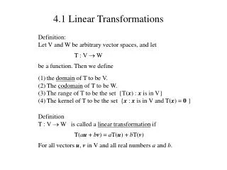
6.1 Introduction to Linear Transformations • A function T that maps a vector space V into a vector space W: V: the domain (定義域) of T W: the codomain (對應域) of T • Image of v under T (在T映射下v的像): If v is a vector in V and w is a vector in W such that then w is called the image of v under T (For each v, there is only one w) • The range of T (T的值域): The set of all images of vectors in V (see the figure on the next slide)
The preimage of w (w的反像): The set of all v in V such that T(v)=w (For each w, v may not be unique) • The graphical representations of the domain, codomain, and range ※ For example, V is R3, W is R3, and T is the orthogonal projection of any vector (x, y, z) onto the xy-plane, i.e. T(x, y, z) = (x, y, 0) (we will use the above example many times to explain abstract notions) ※ Then the domain is R3, the codomain is R3, and the range is xy-plane (a subspace of the codomian R3) ※ (2, 1, 0) is the image of (2, 1, 3) ※ The preimage of (2, 1, 0) is (2, 1, s), where s is any real number
Ex 1: A function from R2 intoR2 (a) Find the image of v=(-1,2) (b) Find the preimage of w=(-1,11) Sol: Thus {(3, 4)} is the preimage of w=(-1, 11)
Addition in V Addition in W Scalar multiplication in V Scalar multiplication in W • Notes: (1) A linear transformation is said to be operation preserving (because the same result occurs whether the operations of addition and scalar multiplication are performed before or after the linear transformation is applied) (2) A linear transformation from a vector space into itself is called a linear operator (線性運算子)
Ex 2: Verifying a linear transformation T from R2 into R2 Pf:
Ex 3: Functions that are not linear transformations (f(x) = sin x is not a linear transformation) (f(x) = x2 is not a linear transformation) (f(x) = x+1 is not a linear transformation, although it is a linear function)
Notes: Two uses of the term “linear”. (1) is called a linear function because its graph is a line (2) is not a linear transformation from a vector space R into R because it preserves neither vector addition nor scalar multiplication
Zero transformation (零轉換): • Identity transformation (相等轉換): • Theorem 6.1: Properties of linear transformations (T(cv) = cT(v) for c=0) (T(cv) = cT(v) for c=-1) (T(u+(-v))=T(u)+T(-v) and property (2)) (Iteratively using T(u+v)=T(u)+T(v) and T(cv) = cT(v))
Ex 4: Linear transformations and bases Let be a linear transformation such that Find T(2, 3, -2) Sol:
Ex 5: A linear transformation defined by a matrix The function is defined as Sol: (vector addition) (scalar multiplication)
Theorem 6.2: The linear transformation defined by a matrix Let A be an mn matrix. The function T defined by is a linear transformation from Rn into Rm • Note: ※ If T(v) can represented by Av, then T is a linear transformation ※ If the size of A is m×n, then the domain of T is Rn and the codomain of T is Rm
Ex 7: Rotation in the plane Show that the L.T. given by the matrix has the property that it rotates every vector in R2 counterclockwise about the origin through the angle Sol: (Polar coordinates: for every point on the xy-plane, it can be represented by a set of (r, α)) r:the length of v( ) :the angle from the positive x-axis counterclockwise to the vectorv T(v) v
according to the addition formula of trigonometric identities (三角函數合角公式) r:remain the same, that means the length of T(v) equals the length of v +:the angle from the positive x-axis counterclockwise to the vector T(v) Thus, T(v) is the vector that results from rotating the vector v counterclockwise through the angle
Ex 8: A projection in R3 The linear transformation is given by is called a projection in R3 ※ In other words, T maps every vector in R3 to its orthogonal projection in the xy-plane, as shown in the right figure
Ex 9: The transpose function is a linear transformation from Mmn into Mnm Show that T is a linear transformation Sol: Therefore, T (the transpose function) is a linear transformation from Mmn into Mnm
Keywords in Section 6.1: • function: 函數 • domain: 定義域 • codomain: 對應域 • image of v under T: 在T映射下v的像 • range of T: T的值域 • preimage of w: w的反像 • linear transformation: 線性轉換 • linear operator: 線性運算子 • zero transformation: 零轉換 • identity transformation: 相等轉換
6.2 The Kernel and Range of a Linear Transformation • Kernel of a linear transformation T (線性轉換T的核空間): Let be a linear transformation. Then the set of all vectors v in V that satisfy is called the kernel of T and is denoted by ker(T) ※ For example, V is R3, W is R3, and T is the orthogonal projection of any vector (x, y, z) onto the xy-plane, i.e. T(x, y, z) = (x, y, 0) ※ Then the kernel of T is the set consisting of (0, 0, s), where s is a real number, i.e.
Ex 1: Finding the kernel of a linear transformation Sol: • Ex 2: The kernel of the zero and identity transformations (a) If T(v) = 0 (the zero transformation ), then (b) If T(v) = v (the identity transformation ), then
Theorem 6.3: The kernel is a subspace of V The kernel of a linear transformation is a subspace of the domain V Pf: T is a linear transformation
Ex 6: Finding a basis for the kernel Find a basis for ker(T) as a subspace of R5 Sol: To find ker(T) means to find all x satisfying T(x) = Ax = 0. Thus we need to form the augmented matrix first
Corollary to Theorem 6.3: • ※ The kernel of T equals the nullspace of A (which is defined in Theorem 4.16 on p.239) and these two are both subspaces of Rn ) • ※ So, the kernel of T is sometimes called the nullspace of T
Range of a linear transformation T (線性轉換T的值域): ※ For the orthogonal projection of any vector (x, y, z) onto the xy-plane, i.e. T(x, y, z) = (x, y, 0) ※ The domain is V=R3, the codomain is W=R3, and the range is xy-plane (a subspace of the codomian R3) ※ Since T(0, 0, s) = (0, 0, 0) = 0, the kernel of T is the set consisting of (0, 0, s), where s is a real number
Theorem 6.4: The range of T is a subspace of W Pf: T is a linear transformation
Notes: (Theorem 6.3) (Theorem 6.4)
Corollary to Theorem 6.4: (1) According to the definition of the range of T(x) = Ax, we know that the range of T consists of all vectors b satisfying Ax=b, which is equivalent to find all vectors b such that the system Ax=b is consistent (2) Ax=b can be rewritten as Therefore, the system Ax=b is consistent iff we can find (x1, x2,…, xn) such that b is a linear combination of the column vectors of A, i.e. Thus, we can conclude that the range consists of all vectors b, which is a linear combination of the column vectors of A or said . So, the column space of the matrix A is the same as the range of T, i.e. range(T) = CS(A)
Use our example to illustrate the corollary to Theorem 6.4: ※ For the orthogonal projection of any vector (x, y, z) onto the xy-plane, i.e. T(x, y, z) = (x, y, 0) ※ According to the above analysis, we already knew that the range of T is the xy-plane, i.e. range(T)={(x, y, 0)| x and y are real numbers} ※ T can be defined by a matrix A as follows ※ The column space of A is as follows, which is just the xy-plane
Ex 7: Finding a basis for the range of a linear transformation Find a basis for the range of T Sol: Since range(T) = CS(A), finding a basis for the range of T is equivalent to fining a basis for the column space of A
Rank of a linear transformation T:V→W (線性轉換T的秩): According to the corollary to Thm. 6.4, range(T) = CS(A), so dim(range(T)) = dim(CS(A)) • Nullity of a linear transformation T:V→W (線性轉換T的核次數): According to the corollary to Thm. 6.3, ker(T) = NS(A), so dim(ker(T)) = dim(NS(A)) • Note: ※ The dimension of the row (or column) space of a matrix A is called the rank of A ※ The dimension of the nullspace of A ( ) is called the nullity of A
Theorem 6.5: Sum of rank and nullity Let T: V →W be a linear transformation from an n-dimensional vector space V (i.e. the dim(domain of T) is n) into a vector space W. Then ※ You can image that the dim(domain of T) should equals the dim(range of T) originally ※ But some dimensions of the domain of T is absorbed by the zero vector in W ※ So the dim(range of T) is smaller than the dim(domain of T) by the number of how many dimensions of the domain of T are absorbed by the zero vector, which is exactly the dim(kernel of T)
Pf: according to Thm. 4.17 where rank(A) + nullity(A) = n ※ Here we only consider that T is represented by an m×n matrix A. In the next section, we will prove that any linear transformation from an n-dimensional space to an m-dimensional space can be represented by m×n matrix
Ex 8: Finding the rank and nullity of a linear transformation Sol: ※ The rank is determined by the number of leading 1’s, and the nullity by the number of free variables (columns without leading 1’s)
Ex 9: Finding the rank and nullity of a linear transformation Sol:
one-to-one not one-to-one • One-to-one (一對一):
Theorem 6.6: One-to-one linear transformation Pf: Due to the fact that T(0) = 0 in Thm. 6.1 T is a linear transformation, see Property 3 in Thm. 6.1
Ex 10: One-to-one and not one-to-one linear transformation because its kernel consists of only the m×n zero matrix because its kernel is all of R3
Onto (映成): (T is onto W when W is equal to the range of T) • Theorem 6.7: Onto linear transformations Let T: V → W be a linear transformation, where W is finite dimensional. Then T is onto if and only if the rank of T is equal to the dimension of W The definition of onto linear transformations The definition of the rank of a linear transformation
Theorem 6.8: One-to-one and onto linear transformations Pf: According to the definition of dimension (on p.227) that if a vector space V consists of the zero vector alone, the dimension of V is defined as zero
Ex 11: = dim(range of T) = # of leading 1’s Sol: If nullity(T) = dim(ker(T)) = 0 If rank(T) = dim(Rm) = m = dim(Rn) = n = (1) – (2) = dim(ker(T))
Isomorphism (同構): • Theorem 6.9: Isomorphic spaces (同構空間) and dimension Two finite-dimensional vector space V and W are isomorphic if and only if they are of the same dimension Pf: dim(V) = n
Since is a basis for V, {w1, w2,…wn} is linearly independent, and the only solution for w=0 is c1=c2=…=cn=0 So with w=0,the corresponding v is 0, i.e., ker(T) = {0} By Theorem 6.5, we can derive that dim(range of T) = dim(domain of T) – dim(ker(T)) = n –0 = n = dim(W) Since this linear transformation is both one-to-one and onto, then V and W are isomorphic
Note Theorem 6.9 tells us that every vector space with dimension n is isomorphic to Rn • Ex 12: (Isomorphic vector spaces) The following vector spaces are isomorphic to each other
Keywords in Section 6.2: • kernel of a linear transformation T: 線性轉換T的核空間 • range of a linear transformation T: 線性轉換T的值域 • rank of a linear transformation T: 線性轉換T的秩 • nullity of a linear transformation T: 線性轉換T的核次數 • one-to-one: 一對一 • onto: 映成 • Isomorphism (one-to-one and onto): 同構 • isomorphic space: 同構空間