Download
1 / 31
310 likes | 472 Views
Economics 101 – Section 5. Lecture #18 – March 25, 2004 Chapter 8 Perfect Competition Competition in the Short-Run. Lecture Overview. Review from last class 3 characteristics of a perfectly competitive market The perfectly competitive firm Example with wheat production

E N D
Economics 101 – Section 5 Lecture #18 – March 25, 2004 Chapter 8 Perfect Competition Competition in the Short-Run
Lecture Overview • Review from last class • 3 characteristics of a perfectly competitive market • The perfectly competitive firm • Example with wheat production • Deriving the short-run supply curve • Long-run equilibrium
Perfect Competition • Perfect competition has 3 important characteristics associated with its market structure • 1) There are a large number of buyers and sellers – each buys or sells only a very small portion of the total quantity in the market • 2) Sellers offer a standardized product • 3) sellers can easily enter or exit the market – no restrictions to entry or exit
The perfectly competitive firm • The goal of a perfectly competitive firm is still to maximize their profit • The perfectly competitive firm faces a cost constraint like any other firm • The cost of producing any given level of output depends on the firms production technology and the prices it must pay for inputs
$400 Demand Curve Facing the Firm Figure 1 The Competitive Industry and Firm (a) (b) Market Firm Price Price per per Ounce Ounce S $400 D Ounces of Ounces of Gold per Day Gold per Day
The perfectly competitive firm • In perfect competition the firm is a price taker • It treats the price of its output as given
(a) Dollars TR TC $2,800 Maximum Profit 2,100 per Day = $700 Slope = 400 550 1 2 3 4 5 6 7 8 9 10 Ounces of Gold per Day (b) Dollars MC d = MR $400 1 2 3 4 5 6 7 8 9 10 Ounces of Gold per Day Figure 2 Profit Maximization in Perfect Competition
The perfectly competitive firm • For a perfectly competitive (PC) firm, the market price is their marginal revenue • Remember that in a PC firm no one supplier can affect the market price by supplying either more or less of the given product • This is why the marginal revenue curve and the demand curve facing the firm are the same • For a PC firm the MR curve is a horizontal line at the market price (where price is on the vertical axis and quantity is on the horizontal axis as is the usual case)
The perfectly competitive firm • Note that this is different from the example used in an earlier lecture • With the example of bed frames the firm could affect the market price by increasing or decreasing their production
The perfectly competitive firm • Finding the profit maximizing level of output for a firm in a PC market utilizes the same rule as we discussed in earlier lectures – • 1) equating MR=MC or • 2) the total revenue and total cost approach • How do we measure total profit? • Graphically • Profit per unit multiplied by the amount sold
(a) Dollars TR TC $2,800 Maximum Profit 2,100 per Day = $700 Slope = 400 550 1 2 3 4 5 6 7 8 9 10 Ounces of Gold per Day (b) Dollars MC d = MR $400 1 2 3 4 5 6 7 8 9 10 Ounces of Gold per Day Figure 2 Profit Maximization in Perfect Competition
The perfectly competitive firm • Profit per unit = P-ATC • Firms will earn a positive profit when P>ATC • This is the rectangle with height P-ATC and length of Q • The firm will incur a loss when P<ATC • This is the rectangle with height ATC-P and length of Q
(b) Economic Loss (a) Economic Profit Dollars Dollars ATC Profit per MC MC Loss per Ounce Ounce $100 $100 d = MR ATC $400 $300 300 d = MR 200 1 2 3 4 5 6 7 8 9 10 1 2 3 4 5 6 7 8 9 10 Ounces of Ounces of Gold per Day Gold per Day Figure 3 Measuring Profit or Loss
The perfectly competitive firm • As the price of output changes, the firm will move along the MC curve in deciding how much it could produce • However if the price is too low and the firm is suffering losses which are large enough then the firm should shut down • Recall that a firm should shut down if it cannot cover its average variable costs (AVC)
The perfectly competitive firm • Recall the following properties from last day: • In the short-run do not shut down if: • TR>TVC • In the short-run shut down if: • TR<TVC • Note Q*P=TR and AVC*Q=TVC • So we continue to operate if P>AVC • Shut down if P<AVC
The perfectly competitive firm • The firms supply curve is not going to be continuous • The firms supply curve can be constructed according to two rules: • 1) If P>AVC then the supply curve is the MC curve • 2) If P is less than the lowest point on the AVC curve, then the supply curve will be a vertical line from zero to this minimum price
Competitive Markets in the SR • Market supply curve • Is the horizontal summation of the individual firm supply curves • Simply add up the quantities of output supplied by all firms in the market at each price
Competitive Markets in the SR • Short-run equilibrium • We have talked about equilibrium in earlier chapters and lectures • This is going to be where the market supply intersects the market demand • Recall market demand was the horizontal summation of individual consumer demand curves (the total amount that would be demanded by a group of consumers at any given price)
Competitive Markets in the SR • What is going on for individual firms when there are changes in the market price? • Would obviously think that as prices go down then firms are going to be worse off? • Why? Because they are getting less $ • How does this tie into their cost structure and all these weird graphs we have been using?
Loss per Bushel at p = $2 2.00 2.00 d 2 D 2 4,000 400,000 Figure 7 Short-Run Equilibrium in Perfect Competition (a) (b) Market Firm Dollars Price per MC ATC S Bushel $3.50 d $3.50 1 Profit per Bushel at p = $3.50 D 1 7,000 Bushels 700,000 Bushels per Year per Year
Competitive markets in the Long-run (LR) • What happens to firms that are making profits in the short-run? Those making losses? • In short, • if there is profit more firms will enter • If there is loss, firms will exit the industry • In a competitive market, economic profit and loss are the forces driving long-run change • The expectation of continued economic profit causes outsiders to enter the market, the expectation of continued economic losses causes firms in the market to exit
Competitive markets in the Long-run (LR) • Long-run equilibrium • If there were profits in the short-run (SR) then entry will shift the market supply to the right until profits are eroded • If there were losses in the SR then exit will cause the market supply to shift left until there are no there are no longer any losses.
Price S 1 per Bushel With initial A supply curve S , market $4.50 1 price is $4.50 . . . D 900,000 Bushels per Year FIGURE 8a From Short-Run Profit to Long-Run Equilibrium
Dollars MC A $4.50 d 1 ATC . . . so each firm earns an economic profit 5,000 9,000 Bushels per Year FIGURE 8b From Short-Run Profit to Long-Run Equilibrium
Price per Profit attracts Bushel entry, shifting the S supply curve 1 rightward . . . S 2 A $4.50 E 2.50 D 900,000 1,200,000 Bushels per Year FIGURE 8c From Short-Run Profit to Long-Run Equilibrium
. . . until market price falls to $2.50 and each firm earns zero economic profit MC ATC A $4.50 d 1 2.50 d 2 5,000 9,000 Bushels per Year FIGURE 8d From Short-Run Profit to Long-Run Equilibrium