Download
1 / 22
220 likes | 922 Views
Background. The pre-solar grain being imaged came from the meteorite MurchisonMurchison hit the Earth on September 28, 1969 in Australia1 . Oak Ridge National Lab. In the summer of 2006, Dr. Phil Fraundorf and Eric Mandell went to Oak Ridge to take Scanning Transmission Electron Microscope (STEM) imagesThe resolution of the Oak Ridge STEM is in the sub-Angstrom (10-10 m) range, and it may be possible to resolve single, heavy atoms.

E N D
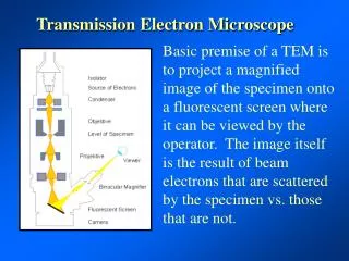
1. Interpreting Images from a Transmission Electron Microscope C. Zak Jost
University of MO � St. Louis
2. Background The pre-solar grain being imaged came from the meteorite Murchison
Murchison hit the Earth on September 28, 1969 in Australia1
3. Oak Ridge National Lab In the summer of 2006, Dr. Phil Fraundorf and Eric Mandell went to Oak Ridge to take Scanning Transmission Electron Microscope (STEM) images
The resolution of the Oak Ridge STEM is in the sub-Angstrom (10-10 m) range, and it may be possible to resolve single, heavy atoms
4. Knowledge Gathered Using intensities of the gray values on the images, data concerning the shape and thickness of the specimen can be inferred
It may be possible to approximate the Z-value of single, heavy atoms
5. Why is this Knowledge Desirable? By locating the respective positions of heavy atoms, one could gather more data concerning how the material formed and what the environment it came from was like
If the heavy atoms could be identified and it could be concluded that they were not due to contamination, this could be a quick and non-destructive way to measure abundances
6. Microscope Detectors The two experimental images analyzed for this project came from the Bright Field (BF) and Dark Field (DF) detectors
The BF gives information about the amount of un-scattered electrons
The DF gives information about scattered electrons
7. Microscope Detectors (cont.) The electron probe scans rows of the specimen
At the same point in time, each detector records their respective currents into images, resulting in two simultaneous experiments
8. Dark Field Image Since the brightness of a pixel increases with the number of protons encountered on the specimen at that point, a graph of intensity should give a qualitative idea of relative thickness
9. Dark Field Intensity Plot
10. Simulated DF Images To test this hypothesis, I generated an atom position list
I then used a program by Kirkland2 to simulate BF and DF images from these atom coordinates
11. Intensity Plots of Simulated Images Using MatLab again, I plotted intensity versus position as in the Experimental DF Image
Notice the correlation of thickness and intensity, with the peaks representing the position of the heavy atoms
12. Comparison of Atom Position and Intensity Plots
13. Profile Plot of Simulated Image A more quantitative way to measure relative thickness is to plot the profile of the region of interest
Notice the same �V� shape as seen before
14. Calculating Absolute Thickness One possibility for getting approximations of absolute thickness is using an equation involving the Mean Free Path: I = Ioe-t / ?
Since the image contains a region with no specimen, the intensity of this region in the BF image is related to the incident electrons, Io.
Using the simulated image, I calculated ? since the thickness, t, was known
15. Bright Field Image
16. Applying MFP Equation to BF Image Getting a list of intensity versus position, I solved the equation for t, and plotted the results
17. Comparison between BF thickness and DF intensity plots Notice the correlation between the intensity plot of the DF image, which has shown to be a good measure of relative thickness, to the absolute thickness plot made from the BF image
18. Z � Value Approximations Though this is a work in progress, some simulation work has been done to show the relationship between scattering and Z-value
19. Scattering versus Z Though the simulations only used three different heavy atoms, the trend line uses the power of about 1.7, which has been shown to be a reasonable relation from previous efforts
By getting the total scattering due to a heavy atom from subtracting the background, one could use this relationship to get approximations of relative Z values
20. Z-value and Thickness If one could get an accurate relationship between Z-value and scattering, the thickness could be calculated by solving for the number of particles (N) in the following equation:Intensity = N*const*Z1.7
The constant would be determined by simulation or other means
21. Future Explorations Work is currently being done to use a mean-free-path equation to get an independent Z-value approximation
More simulations are being ran that test whether the BF aperture size affects the mean free path
22. Summary Intensity plots of Dark Field images provide a good qualitative understanding of relative thickness and heavy atom positions
A mean-free-path equation applied to the Bright Field image gives an approximate value of absolute thickness if there is a region in the image with no specimen
It might be possible to infer approximations of Z-value of single heavy atoms from the intensity in Dark Field images
The Z-value approximation may independently give values to thickness, which can be compared to the mean-free-path method