Solving NMR structures Part I: Experimentally derived restraints
340 likes | 789 Views
Solving NMR structures Part I: Experimentally derived restraints. 1. Distance restraints from crosspeak intensities in NOESY spectra; measuring and calibrating NOEs 2. Dihedral angle restraints from three-bond J couplings; measuring J couplings; chemical shifts and dihedral angles

Solving NMR structures Part I: Experimentally derived restraints
E N D
Presentation Transcript
Solving NMR structures Part I:Experimentally derived restraints 1. Distance restraints from crosspeak intensities in NOESY spectra; measuring and calibrating NOEs 2. Dihedral angle restraints from three-bond J couplings; measuring J couplings; chemical shifts and dihedral angles 3. Hydrogen bond restraints from amide hydrogen exchange protection data 4. Orientational restraints from residual dipolar couplings (covered in a separate lecture)
1. Using NOESY to generate nOe distance restraints • NOESY measurements are not steady-state nOe’s: we are not saturating one resonance with constant irradiation while observing the effects at another. • Instead, we are pulsing all of the resonances, and then allowing nOe’s to build up through cross-relaxation during a mixing time --so nOe’s in a NOESY are kinetic: crosspeak intensities will vary with mixing time • typical tm’s used in an NOESY will be 20-200 ms. from Glasel & Deutscher p. 354 mixing time basic NOESY pulse sequence
nOe buildup in NOESY • other things being equal, the initial rateof buildup of a NOESY crosspeak is proportional to 1/r6, where r is the distance between the two nuclei undergoing cross-relaxation. • nOe buildup will be faster for larger proteins, which have a longer correlation time tc, and therefore more efficient zero-quantum cross-relaxation • initially crosspeak intensity builds up linearly with time, but then levels off, and at very long mixing time will actually start to drop due to direct (not cross) relaxation.
spin diffusion • under certain circumstances, indirect cross-relaxation pathways can be more efficient than direct ones, i.e. A to B to C more efficient than A to C. This is called spin diffusion • when this happens the crosspeak intensity may not be a faithful reflection of the distance between the two nuclei.
Crosspeaks due to spin diffusion exhibit delayed buildup in NOESY experiments • spin diffusion peaks • are usually observed • at long mixing time, and their intensity does not reflect the initial rate of buildup • these effects can be avoided either by sticking with short mixing times or by examining buildup curves over a range of mixing times
Other nOe caveats • I mentioned that nOe buildup rates are faster for larger proteins because of the longer correlation time • It’s also true that buildup rates can differ for nuclei within the same protein if different parts of the protein have different mobility (hence different correlation times) • for parts of the protein which are relatively rigid (such as the hydrophobic core) correlation times will more or less reflect that of the whole protein molecule--nOe buildup will be fast • disordered regions (at the N- or C-termini, for instance) may have much shorter effective correlation times and much slower nOe buildup as a consequence • the bottom line is, the actual nOe observed between two nuclei at a given distance r is often less than that expected on the basis of the overall molecular correlation time.
The goal: translating NOESY crosspeak intensities into nOe distance restraints • because the nOe is not always a faithful reflection of the internuclear distance, one does not, in general, precisely translate intensities into distances! • instead, one usually creates three or four restraint classes which match a range of crosspeak intensities to a range of possible distances, e.g. classrestraintdescription *for protein w/ Mr<20 kDa strong 1.8-2.7 Å strong intensity in short tm (~50 ms*) NOESY medium 1.8-3.3 Å weak intensity in short tm (~50 ms*) NOESY weak 1.8-5.0 Å only visible in longer mixing time NOESY • notice that the lower bound of 1.8 Å (approximately van der Waals contact) is the same in all restraint classes. This is because, for reasons stated earlier, atoms that are very close can nonetheless have very weak nOe’s, or even no visible crosspeak at all.
Calibration of nOe intensities • the crosspeak intensities are often calibrated against the crosspeak intensity of some internal standard where the internuclear distance is known. The idea of this is to figure out what the maximal nOe observable will be for a given distance. • this calibration can then be used • to set intensity cutoffs for restraint • classes, often using a 1/r6 dependence tyrosine d-e distance always the same! • ideally, one chooses • an internal standard • where the maximal nOe • will be observed (i.e. something not undergoing a lot of motion)
2. Coupling constants and dihedral angles There exist relationships between three-bond scalar coupling constants3Jand the corresponding dihedral anglesq, called Karplus relations. These have the general form 3J = Acos2q + Bcosq + C from p. 30 Evans textbook
Empirical Karplus relations in proteins • comparison of 3J values measured in solution with dihedral angles observed in crystal structures of the same protein allows one to derive empirical Karplus relations that give a good fit between the coupling constants and the angles coupling constants in solution vs. f angles from crystal structure for BPTI these two quantities differ by 60° because they are defined differently from p. 167 Wuthrich textbook
Empirical Karplus relations in proteins • Here are some empirical Karplus relations: 3JHa,HN(f)= 6.4 cos2(f - 60°) -1.4 cos(f - 60°) + 1.9 3JHa,Hb2(c1)= 9.5 cos2(c1- 120°) -1.6 cos(c1- 120°) + 1.8 3JHa,Hb3(c1)= 9.5 cos2(c1) -1.6 cos(c1) + 1.8 3JN,Hb3(c1)= -4.5 cos2(c1+ 120°) +1.2 cos(c1+ 120°) + 0.1 3JN,Hb2(c1)= 4.5 cos2(c1- 120°) +1.2 cos(c1- 120°) + 0.1 • Notice that use of the relations involving the b hydrogens would require that they be stereospecifically assigned (in cases where there are two b hydrogens) • note that these relations involve f or c1 angles
Measuring 3JHN-Ha: 3D HNHA spectra ratio of crosspeak and diagonal peak intensities can be related to 3JHN-Ha J large J small HN to Ha crosspeak HN diagonal peak this is one plane of a 3D spectrum of ubiquitin. The plane corresponds to this 15N chemical shift Archer et al. J. Magn. Reson. 95, 636 (1991).
3D HNHB experiment • similar to HNHA but measures 3JN-Hb couplings instead DeMarco, Llinas, & Wuthrich Biopolymers 17, p. 2727 (1978). for c1 =180 both 3JNb ~1 Hz for c1 =+60,-60 one is ~5, other is ~1 can’t tell the difference unless b’s are stereospecifically assigned
3D HN(CO)HB experiment • complementary to HNHB • measures 3JC,Hbcouplings for a particular b proton, if q=180, 3JC,Hb= ~8 Hz if q=+60 or -60, 3JC,Hb= ~1 Hz Grzesiek et al. J. Magn. Reson. 95, 636 (1991).
HNHB and HN(CO)HB together 3JC,Hb3= small 3JC,Hb2= large 3JN,Hb3= small 3JN,Hb2= small 3JC,Hb3= large 3JC,Hb2= small 3JN,Hb3= small 3JN,Hb2= large 3JC,Hb3= small 3JC,Hb2= small 3JN,Hb3= large 3JN,Hb2= small
HNHB, HN(CO)HB together • can thus get both c1 angle and stereospecific assignments for b’s from a combination of HNHB and HN(CO)HB HNHB HN(CO)HB from Bax et al. Meth. Enzym. 239, 79.
Dihedral angle restraints • derived from measured J couplings • as with nOe’s, one does not translate J directly into a quantitative dihedral angle, rather one translates a range of J into a rangeof possible angles, e.g. 3JHa,HN(f) < 6 Hz f= -65° ± 25° 3JHa,HN(f) > 8 Hz f= -120 ± 40° This accounts for errors in measurement as well as the fact that the Karplus relation itself is not exact.
Chemical shifts and backbone conformation • chemical shifts depend upon local electron distributions, bond hybridization states, proximity to polar groups, nearby aromatic rings, local magnetic anisotropies. • in other words, chemical shifts depend upon the structural environment and thus can provide information about structure • observation of relationships between chemical shifts and protein secondary structure has led to the development of some useful empirical rules • The most common of these rules relate to backbone conformations (combinations of dihedral angles)
Ha chemical shifts and secondary structure • Hachemical shifts are generally lower for a-helices than for b-sheets • the figure at right shows distributions of Ha chemical shifts observed in sheets (lighter bars) and helices (darker bars). The black bar in each distribution is the median. • Hachemical shifts in a-helices are on average 0.39 ppmbelow“random coil” values, while b-sheet values are 0.37 ppm above random coil values. Wishart, Sykes & Richards J Mol Biol (1991) 222, 311.
Chemical shift index (CSI) • trends like these led to the development of the concept of the chemical shift index* as a tool for assigning secondary structure using chemical shift values. • one starts with a table of reference values for each amino-acid type, which is essentially a table of “random coil” Havalues • CSI’s are then assigned as follows: exp’tl Ha shift rel. to referenceassignedCSI within ± 0.1 ppm 0 >0.1 ppm lower -1 >0.1 ppm higher +1 *Wishart, Sykes & Richards Biochemistry (1992) 31, 1647-51.
Chemical shift indices • one can then plot CSI vs. sequence and assign 2ndary str. as follows: • any “dense” grouping of four or more “-1’s”, uninterrupted by “1’s” is assigned as a helix, while any “dense” grouping of three or more “1’s”, uninterrupted by “-1’s”, is assigned as a sheet. • a “dense” grouping means at least 70% nonzero CSI’s. • other regions are assigned as “coil” • this simple technique assigns 2ndary structure w/90-95% accuracy • similar useful relationships exist for 13Ca, 13Cb13CC=O shifts CSI residue #
Here’s a figure showing deviations of Ca and Cb chemical shifts from random coil values when in either a-helix or b-sheet conformation for a-helices, Ca shifts are higher than normal, whereas Cb shifts are lower than normal.
Chemical shifts and structural restraints • CSI is a very widely used technique for quickly and qualitatively assigning secondary structures from chemical shift data. • Restraints on structure for use in explicit structure calculationsare also derivable from chemical shifts, analogous to our nOe-derived distance restraints, our coupling-constant-derived dihedral angle restraints and our hydrogen-exchange derived hydrogen bond restraints. • These restraints often take the form of potential functions. For example, 13Caand 13Cb chemical shifts are determined largely by the backbone angles f and y, so potential functions can be used to restrain these angles to values near to those expected based on the observed shifts. • Such potentials can supplement the use of J-couplings in restraining dihedral angles. • Such potentials are not in very wide use in structure calculations yet and we will not cover them further here. The interested student should see Clore and Gronenborn PNAS (1998) 95, 5891 for a review of this topic.
3. Amide hydrogen exchange and H-bonds half-life exchange rate amide protons undergo acid- and base-catalyzed exchange with solvent protons at a rate which ranges from the second to minute time scale, depending upon solvent conditions (mostly pH) if a protein is placed in D2O, the amide signals due to 1H nuclei will disappear over time due to this exchange poly-D,L-alanine exchange rate in D2O at 20 °C. Minimum with respect to pH is due to the fact that exchange is both acid and base catalyzed pH but in D2O! Englander & Mayne, Ann. Rev. Biophys. Biomol. Struct. (1992) 21, 243.
Amide hydrogen exchange • when amide protons are involved in hydrogen bonds in a folded protein, they are protected from exchange with solvent and thus exchange somewhat more slowly, i.e. faster: N-H --> N-D slower: N-H....O=C --> N-D....O=C
Protection factors • the protection factor Pfor a given amide proton is the intrinsic rate of exchange expected for that amide proton in an unfolded protein under a given set of solvent conditions, divided by the observed rate of exchange in the native state P= kex(U)/kex(N) where U is the unfolded state and N is the native state • intrinsic rates of exchange vary with the amino acid sequence and the solvent conditions in a predictable manner--there are published tables and websites where you can look them up/calculate them.
Measuring amide exchange rates • 15N-1H HSQC spectra are a good way to monitor exchange because individual well-resolved peaks are visible for most amides • one might record a spectrum in H2O, freeze dry the sample, resuspend in D2O, and record a series of spectra in D2O to monitor the rate at which each amide proton disappears picture at left: 15N-1H HSQC of Arc repressor 5 min after resuspension in D2O (pH 4.7)--note that unprotected amides such as the unstructured N-terminus (1-7) have already exchanged. This is because intrinsic half-lives at this pH are in the vicinity of 10 seconds to a minute. Burgering et al. Biopolymers (1995) 35, 217.
The plot above shows measured exchange rates from a series of15N-1H HSQC spectra for Arc repressor. Protected amides are usually within secondary structure elements, but the presence of secondary structure doesn’t guarantee that protection will be observed (note the lack of protection for the beta-sheet from residue 9-14). Lack of protection could indicate that the secondary structure element undergoes fairly rapid local unfolding. Note the strength of NMR and HSQC in particular here--you get a separate exchange rate for every amide proton--great residue-specific dynamic information!
HX (hydrogen exchange) of Syrian hamster prion protein surface is less well-protected ends of helices less well-protected blue spheres: P > 4650 green spheres: 370 < P < 4650 red spheres: P < 370 note that while all protected amides are hydrogen-bonded, not all hydrogen-bonded amides are equally well protected. Rates differ both within secondary structure elements (buried positions near the center usually most protected) and between different secondary structure elements Liu et al.Biochemistry (1999) 38, 5362.
Hydrogen bond restraints • amide protons showing significant protection are inferred to be involved in hydrogen bonds, but it is not clear from this data alone what the identity of the hydrogen bond acceptor group is. • however, if additional information is available, one can infer what the acceptor is. For instance, daN(i-3,i) and daN(i-4,i) nOe’s such as are characteristic of a-helices imply that the protected amide of residue i is hydrogen bonded to the carbonyl of residue i-4. • hydrogen bond restraints are usually expressed as a pair of distance restraints, e.g dHN-O = 1.5-2.3 Å, dN-O = 2.5-3.3 Å. A pair of restraints like this ensures reasonable good geometry for the hydrogen bond.