Download
1 / 29
330 likes | 668 Views
Tools of Oceanography. December 1. Important Quantities to Measure. Density → Temperature, Salinity, Pressure Can infer currents from density distribution Can infer water mass origin from T-S ratio Sea Surface height Currents Waves

E N D
Tools of Oceanography December 1
Important Quantities to Measure • Density → Temperature, Salinity, Pressure • Can infer currents from density distribution • Can infer water mass origin from T-S ratio • Sea Surface height • Currents • Waves • Winds, SST, Humidity, Air Temperature, Barometric Pressure, solar radiation, precipitation
Water samples: get salinity in lab with salinometer • Reversing/Closing Bottles: • Nansen • Niskin • Temperature: • Reversing Thermometer • XBT • Conductivity • Temperature and Salinity with Depth: CTD – Conductivity and Temperature → Salinity • Thermo-salinograph – underway – T & S along ship track
Nansen and Niskin bottles http://www-ocean.tamu.edu/education/oceanworld-old/students/satellites/satellite2.htm http://en.wikipedia.org/wiki/Nansen_bottle
Figure 6.11 Left: Protected and unprotected reversing thermometers is set position, before reversal. Right: The constricted part of the capillary in set and reversed positions. From von Arx (1962).
Platinum Resistance Thermometer: This is the standard for temperature. It is used by national standards laboratories to interpolate between defined points on the practical temperature scale. It is used primarily to calibrate other temperature sensors. Thermistor: A thermistor is a semiconductor having resistance that varies rapidly and predictably with temperature. It has been widely used on moored instruments and on instruments deployed from ships since about 1970. It has high resolution and an accuracy of about ± 0.001°C when carefully calibrated. Bucket temperatures: The temperature of surface waters has been routinely measured at sea by putting a mercury thermometer into a bucket which is lowered into the water, letting it sit at a depth of about a meter for a few minutes until the thermometer comes to equilibrium, then bringing it aboard and reading the temperature before water in the bucket has time to change temperature. The accuracy is around 0.1°C. This is a very common source of direct surface temperature measurements. Ship Injection Temperature: The temperature of the water drawn into the ship to cool the engines has been recorded routinely for decades. These recorded values of temperature are called injection temperatures. Errors are due to ship's structure warming water before it is recorded. This happens when the temperature recorder is not placed close to the point on the hull where water is brought in. Accuracy is 0.5°-1°C.
Figure 6.13 A conductivity cell. Current flows through the seawater between platinum electrodes in a cylinder of borosilicate glass 191 mm long with an inside diameter between the electrodes of 4 mm. The electric field lines (solid lines) are confined to the interior of the cell in this design making the measured conductivity (and instrument calibration) independent of objects near the cell. This is the cell used to measure conductivity and salinity shown in Figure 6.15. From Sea-Bird Electronics.
Navigation: • Loran – good to 100m near shore – 500 km offshore • GPS – satellite navigation system • Good to 2 m, to a few cm in differential mode http://www.colorado.edu/geography/gcraft/notes/gps/gps_f.html
Navigation: • Loran – good to 100m near shore – 500 km offshore • GPS – satellite navigation system • Good to 2 m, to a few cm in differential mode • Current: • Mechanical Current meters – Rotor and Vane, inclinometer • E-M • Acoustic
Mechanical Current Meters The Ekman Current Meter had an impeller and vane for direction. The Vector Measuring Current Meter, VMCM, has two fans which break the current into north and east components. It also has a temperature sensor on board, and some have a conductivity cell to determine salinity. Ekman CM VMCM
HOW THE ADCP WORKS: A Sontek figure showing what happens to the frequency of sound waves when they reflect off of moving objects. (from YSI/Sontek) http://www.whoi.edu/instruments/viewInstrument.do?id=819
Lagrangian Drifters – surface and subsurface Sub-surface drag created by “drogue” to make sure drifter follows water
Satellites – synoptic coverage - global Polar orbiting – see swaths of earth’s surface a few times a day at higher resolution (as high as a few meters to 1 km) Geosynchronous orbits – see entire hemisphere at lower resolution (~10 km at nadir)
Advanced Very High Resolution Radiometer (AVHRR) for SST – on NOAA polar orbiters • Uses multiple wavelengths in IR and near-IR • HRPT: High Resolution Picture Trans. – 1 km resolution • GAC: Global Ave. Coverage – 4 km resolustion • LAC: Local Area Coverage – 1 km • Pre-programmed for special areas of interest • Sees only upper 1 mm temperature – may or may not indicate mixed-layer temperature depending on mixed-layer dynamics • Can’t see thru clouds
Ocean Color: • CZCS: 1978-1986 • SeaWiFS – Sea-viewing Wide Field-of-view Sensor – 1997-present • MODIS (Aqua, Terra) • Altimetry: • GEOSAT/SeaSat • TOPEX/Poseidon – 17 day repeat orbit • Scatterometer Winds – NSCAT, ERS, QuickScat
Ocean Models • Use computers to solve numerical approximation to Equations of Motion • Approximate derivatives numerically • u(x,y,z,t) = u(i dx, j dy, k dz, n dt) = u(i,j,k,n) • same for other variables • Express derivative terms in Finite Differences:
Equation like Become in finite differences Use information from the past (time step n-1) and the present (time step n) to predict the future (time step n+1)
Finite difference schemes – stability, CFL For stability, waves must not travel more than one grid cell in in one time step C dt/dx < 1 Called CFL Condition Horizontal resolution (dx, dy) determines time step Horizontal resolution determined by scale of features to be reproduced Time step and resolution determine computational load
Types of models: Finite element vs. Finite difference Layer vs. Level Sigma coord. Vs. Z-level POM/ECOM/ROMS/EFDC: Sigma coord. GFDL/MOM: z- level MICOM/Reduced Gravity models: Isopycnic HYCOM: Hybrid QUODDY/ADCIRC: Finite Element
Z-level coordinates: dz is fixed - useful for deep ocean, boundary layers Sigma-coordinates – follow bathymetry – useful for coastal and estuarine models where z = h (x, y, t) is the sea surface, and z = -H (x, y) is the bottom Isopycnic coordinates: use density surfaces as vertical coordinate Reduced Gravity Models are subset of Isopycnic models, where lowest layer is assumed motionless - like Level of No Motion in Geostrophic Method
The Tampa Bay Model (ECOM3D): Grid: 70 x 100 x 10 - 22,440 active cells - 300 m to 2200 m resolution Time step: 60 sec. Bathymetry from NGDC/GEODAS 4.0 Driven by: Observed winds Water level, Temperature/Salinity @ Egmont Key Precipitation estimated from 68 to 80 SWFWMD rain gages (Daily) Evaporation estimated from observed winds, atmospheric humidity, and water surface temperature Streamflow estimated from USGS gages, SWFWMD drainage basins, and municipal point sources at 34 inflow ports (Daily) Calibrated/Validated against EPC and TOP salinities, PORTS and TOP water level and velocity Hindcast, Nowcast/Forecast Modes
Millions of grid cells times millions of time steps- What to do with all that output? Sample like “real” ocean data – maps, sections, time series Visualization – animations, fly-thru’s
Animation of sea surface height from the NRL 1/4° global, 6 layer finite depth hydrodynamic model, viewed from the equator.
Animation of sea surface height from the NRL 1/4° global, 6 layer finite depth hydrodynamic model, viewed from over the south pole